
In this tutorial, the basic steps of working with DynamO are introduced by performing a simulation of a hard sphere fluid.
You will need to have access to an installed copy of DynamO, either by using the precompiled packages in the download section of the site or by following the previous tutorial to compile and install your own copy of DynamO. You can check if dynamo works by opening a terminal and typing the following command:
dynamodIf everything is working correctly, you should see the copyright notice and the descriptions of the options of the dynamod program:
dynamod  Copyright (C) 2013  Marcus N Campbell Bannerman
This program comes with ABSOLUTELY NO WARRANTY.
This is free software, and you are welcome to redistribute it
under certain conditions. See the licence you obtained with
the code
Usage : dynamod <OPTIONS>...[CONFIG FILE]
...
If you do not see the above output, please double check that you encountered no errors while installing/building DynamO. If you have problems and you have built DynamO yourself, you can return to the previous tutorial and recheck the output of the make command.
When performing a molecular dynamics simulation with DynamO, the standard steps, or "workflow", is to:
This tutorial will give you a general understanding of these steps.
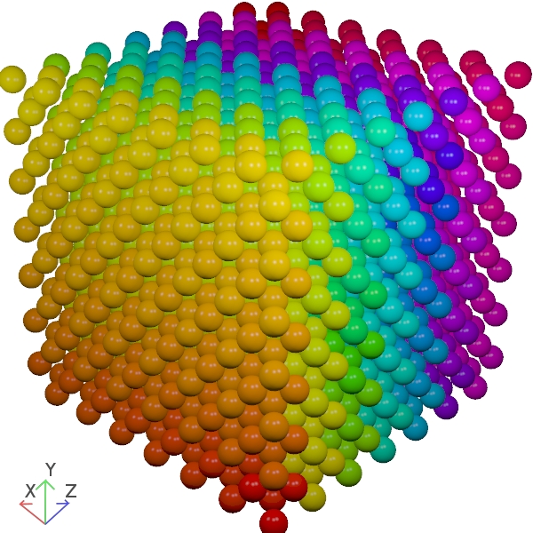
A video of the hard sphere system which is generated and simulated in this tutorial.
In this tutorial you will simulate a hard-sphere fluid. The hard sphere is a simple molecular model used to capture the fundamental effects of "excluded-volume" interactions (see the reference entry for more details). A video of the initial configuration and equilibration performed in this tutorial is presented below. At the start of the video, the hard spheres are shown in their initial configuration. The particles are placed on a lattice and assigned random velocities. The particles are then coloured by their ID number and the simulation is "run".
Here we use periodic boundary conditions as they allow us to simulate a small amount of fluid as though it is part of an infinite/bulk system (see the reference entry for more details).
As the simulation proceeds, the initial lattice structure rapidly disappears. However, it is obvious from the clear colour banding that the particles have not actually moved very far from their initial positions. The system still has a configurational "memory" of its initial state. If we're trying to measure the ensemble average of properties, like the diffusion coefficient, we will need to ensure that the initial state has no effect on the results collected.
To equilibrate the system and move it away from this initial state, the simulation is then set to run at full speed for a few thousand collisions and then slowed down again to take a look at the results. We can see that the simulation has equilibrated well and the coloured particles are well mixed. This system should now be ready to sample "equilibrium"/ensemble-average data from.
Let's take a look at how this simulation was performed in DynamO...
There are only three commands to cover in this tutorial, so we'll cover them briefly and then go into each command in detail.
Let us say that you want to run a hard-sphere simulation of 1372 particles. These particles should be packed together at a reduced density of 0.5 and have a reduced temperature of 1 (if these values look peculiar, please see the FAQ on the units of DynamO). You want to create the system, and then run it for $10^6$ collisions to equilibrate, then carry on and run it for another $10^6$ collisions to collect some data. All you have to do is run the following commands in your terminal/shell:
dynamod -m 0 -C 7 -d 0.5 --i1 0 -r 1 -o config.start.xml
dynarun config.start.xml -c 1000000 -o config.equilibrated.xml
dynarun config.equilibrated.xml -c 1000000 -o config.end.xml
We'll look at each command individually in the following sections.
The first step in the brief example was to create the initial configuration file, called config.start.xml, using dynamod.
dynamod -m 0 -C 7 -d 0.5 --i1 0 -r 1 -o config.start.xmlIn this section, we will briefly learn about the configuration files of DynamO, which are the main input and output of DynamO, and how to generate configuration files using dynamod.
Before we can run any simulations with DynamO, we must write or generate a configuration file. A configuration file is a single file which contains all of the parameters of the system and it is used for...
Every single parameter of the system is set in a configuration file, including the particle positions, interactions, boundary conditions and solver details. Many other simulation packages usually place some of this information in several different files, but DynamO only uses one file. This means there is a lot of information in this one file and it can be quite difficult to generate from scratch. So lets take a look at how we can generate an basic example configuration file to start us off.
dynamod is a program designed to generate example configuration files, or to manipulate existing configuration files. We can take a look at the options of dynamod using the --help option:
dynamod --helpThere are many options available and a lot are related to modifying existing configurations (this is why it is called dynamod), but if we want to generate a configuration we are only need to be interested in the bottom section which starts with:
...
Packer options:
  -m [ --pack-mode ] arg    Chooses the system to pack (construct)
                            Packer Modes:
                            0:  Monocomponent hard spheres
                            1:  Mono/Multi-component square wells
                            2:  Random walk of an isolated attractive polymer
...
This section is a list of the built in example configurations that dynamod can produce. We ask dynamod to generate any one of the configurations listed there using the --pack-mode option (or -m for short).
As this is a tutorial on hard spheres, we will want to use mode 0. Once you have selected your --pack-mode, you can request more information on its specific options by using the --help option again in combination with the selected --pack-mode:
dynamod -m0 --helpAnd you should get the following output:
Mode 0: Monocomponent hard spheres
 Options
  -C [ --NCells ] arg (=7)    Set the default number of lattice unit-cells in each direction.
  -x [ --xcell ] arg          Number of unit-cells in the x dimension.
  -y [ --ycell ] arg          Number of unit-cells in the y dimension.
  -z [ --zcell ] arg          Number of unit-cells in the z dimension.
  --rectangular-box           Set the simulation box to be rectangular so that the x,y,z cells also specify the simulation aspect ratio.
  -d [ --density ] arg (=0.5) System density.
  --i1 arg (=FCC)             Lattice type (0=FCC, 1=BCC, 2=SC)
  --i2 arg (disabled)         Adds a temperature rescale event every x events
  --f1 arg (=1.0)             Sets the elasticity of the hard spheres
What you can see here are a list of options with their default values in parenthesis, so if you run:
dynamod -m0 -o config.start.xml.bz2It will actually output the same result as running the following command.
dynamod -m 0 -C 7 -d 0.5 --i1 0 -r 1 -o config.start.xmlThis is the exact command that was discussed in the brief overview, and its the default set-up of the hard-sphere example. There are lots of options you can use to change the density, number of particles and their placement, and these are discussed in the next section.
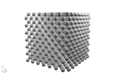
The default FCC hard sphere system generated by dynamod.
Most of the options for this --pack-mode (and many other pack modes) control the initial placement of the particles.
When you create an initial configuration, you must be careful to place the particles so that there are no overlaps which would lead to invalid dynamics. If we placed two hard sphere particles so that they were overlapping, the system would be in an invalid state as "hard" particles cannot interpenetrate each other. On the other hand, we want to be able to "pack" the particles as close together as possible so that we can generate high density configurations easily. Obviously we cannot just randomly drop particles as this will quickly lead to overlaps, even in low density systems.
What we're looking for is a regular structure, or lattice, which maximises the distance between the different positions, or "sites", for a fixed size of system. This structure would ensure that we minimise the chance of any particles overlapping right at the start of the simulation. Such structures occur frequently in nature and they're called crystal lattices. You can take a look at Wikipedia's article on the closest way to pack spheres for more information on this topic.
For mono-sized spheres, there are three popular cubic crystal structures which are used by simulators to initially position particles. There is Face-Centred Cubic (FCC), Body-Centered Cubic (BCC), and the Simple (or Primitive) Cubic (SC). DynamO can use any of these three to initially place your particles, and this is selected using the first integer argument (--i1 X, where X=0 for FCC, X=1 for BCC and X=2 for SC).
The FCC crystal often is favoured for producing the initial particle positions as it is the naturally-forming crystal structure of single-sized hard-spheres. Thus, it gives the closest packing you can physically achieve for mono-sized hard spheres without generating overlaps. It also provides a good starting point for other particle shapes and types too, so you'll often see rods, polymers, and other shapes initially arranged in an FCC lattice.
So, back to dynamod. When you pass -C7 --i1 0 to dynamod you are asking dynamo to produce a $7\times7\times7$ (-C 7) FCC (--i1 0) lattice and place a single particle on each lattice site.
As the FCC lattice has 4 unique sites per unit cell, this will result in $N=4\times7^3=1372$ particles being generated. The size of the particles is then scaled to match the density passed using the --density option, or -d for short (by default we have -d 0.5).
To conclude this part, we'll quickly summarise the description of each of the options passed to dynamod:
dynamod -m 0 -C 7 -d 0.5 --i1 0 -r 1 -o config.start.xmlThe above command says:
When you run this simulation you will get a lot of text on the screen detailing the steps dynamod is carrying out, but at the end you should see the following
Simulation: Config written to config.start.xml
Which indicates the command was successful. You can take a look at the contents of the configuration file, but the configuration file will be explained in more detail in the next tutorial.
The most complex part of this tutorial is now over. All that remains is to take this initial starting configuration file and actually run a simulation.
The running of simulations is performed using the dynarun command. This command has many options which can be listed using the --help option, but for now we'll only use the -c and -o options. The command we're going to use is:
dynarun config.start.xml -c 1000000 -o config.equilibrated.xmlThis command takes the configuration in config.start.xml and runs it for 106 events/collisions (-c 1000000), before putting the final configuration in config.equilibrated.xml. We specify the duration of the simulation in events as DynamO is an event-driven simulator, and the natural unit of computation is an event. You may specify the duration in units of time using the -h option like so:
dynarun config.start.xml -f 190 -o config.equilibrated.xmlIn this system, a simulation for 190 units of time is roughly proportional to $10^6$ events, so both commands should result in roughly the same simulation duration. Its just more natural to specify the duration in events (collisions) as the simulator processes these at a constant rate.
When you run the command above, you should see some periodic output from dynarun informing you of its progress in the simulation:
ETA 15s, Events 100k, t 19.0566,0.130728, T 1, U 0 ETA 14s, Events 200k, t 38.0891, 0.130645, T 1, U 0 ...
In order, the columns are: an estimate of how much longer the simulation will take (ETA), how many events have been executed already, and how much simulation time has passed. The average mean free time (MFT), the average temperature (T) and configurational internal energy (U) are also outputted to help you track the equilibration of the system. These values should fluctuate around a fixed value once the system reaches equilibrium. Once the simulation is over, you'll see that the final configuration is written out to config.equilibrated.xml:
Simulation: Output written to output.xml.bz2
Simulation: Config written to config.equilibrated.xml
Some collected data is also written to output.xml.bz2, but this data will contain influences of the initial crystalline configuration so it should be discarded. The purpose of this first run is to allow the system to have enough time to "relax" from this crystalline configuration and "forget" about this initial configuration. Ideally, our results should be the same regardless of where we started (a property of systems which are ergodic).
From previous experience, $10^6$ events is more than enough to equilibrate this small system of 1372 particles. If we were uncertain about the equilibration of this system, we might monitor the mean free time (and other properties) and check they reach a steady value. The final configuration from this "equilibration" run is now used as the input to a new "production" run using the following command:
dynarun config.equilibrated.xml -c 1000000 -o config.end.xmlSimulation: Output written to output.xml.bz2 Simulation: Config written to config.end.xml
The final configuration is written out to the config.end.xml file, but this is not the only source of data outputted by the dynarun command. In the following section we discuss the contents of the output.xml.bz2 file.
If you want to visualise a configuration or simulation, you replace the dynarun program with the dynavis program like so:
dynavis config.equilibrated.xml -c 1000000 -o config.end.xmlThe simulation will load and the visualiser windows will appear. The simulation will be paused at the start and you can un-pause it using the visualiser controls. If you close the visualiser windows, the simulation will automatically unpause and will carry on running.
dynarun has the ability to collect a wide range of properties for molecular and granular systems. These include complex properties such as transport coefficients (viscosity, thermal conductivity, and mutual/thermal diffusion) along with more traditional properties such as radial distribution functions, power loss, pressure tensors and much more (see the output plugin reference for more details). Some analysis of the more complex properties will be covered in the following tutorials, but there are some basic properties which we'll cover in this tutorial.
Any data collected on the simulation by dynarun is outputted to a compressed XML file called output.xml.bz2 (you can change the output file name using the --out-data-file option). Both the configuration files and the output files are written in XML, as it is a format that is easy for both humans and computers to read. We'll cover how to look at this data by hand now, but this data format is also easy for a computer to read (see Appendix A: Parsing Output and Config Files).
To read this output data file, you must first un-compress the file using the bunzip2 command using the following command:
bunzip2 output.xml.bz2This will uncompress the file from output.xml.bz2 into output.xml, and you will be able to open it using your favourite text editor. Even internet browsers can open XML files and an example output.xml file from the default hard sphere simulation is available at the link below.
Taking a look inside output.xml, we can see there's lots of information available. The mean free time, density, packing fraction, particle count, simulation size, memory usage and performance are available. The temperature is available too:
<Temperature Mean="1.00000000000009" MeanSqr="1.00000000000008" Current="1" Min="1" Max="1"/>
Here you can see that the temperature is almost exactly 1. Hard spheres have no configurational internal energy, so once you set their temperature in an NVE simulation it will not fluctuate.
A more interesting property for the hard sphere system is the pressure, conveniently available under the Pressure tag:
<Pressure Avg="1.63556218044793">
  <Tensor>
1.63441469271575 0.000297605402684329 -0.00208381219921736
0.000297605402684328 1.6372827542425 -0.00132202770190308
-0.00208381219921736 -0.00132202770190307 1.63498909438556
  </Tensor>
  <InteractionContribution>
1.13429624862172 7.16513124308423e-05 -0.00117809530934935
7.16513124308414e-05 1.13722663976942 -0.00126595577928373
-0.00117809530934935 -0.00126595577928373 1.13516365295252
  </InteractionContribution>
</Pressure>
The hydraulic pressure, $p=\left(P_{xx}+P_{yy}+P_{zz}\right)/3$, is available as the Avg attribute of the Pressure tag, but the full pressure tensor, $\mathbf{P}$, is enclosed in the Tensor tags. The pressure values are just written out as a set of space separated values which are arranged as follows:
$$ \begin{align} \mathbf{P}= \begin{pmatrix} P_{xx} & P_{xy} & P_{xz}\\ P_{yx} & P_{yy} & P_{yz}\\ P_{zx} & P_{zy} & P_{zz} \end{pmatrix} \end{align} $$More information on the pressure tag is available in the reference documentation for the Pressure tag:
There are some other properties available, such as the configurational internal energy and residual heat capacity:
<UConfigurational Mean="0" MeanSqr="0" Current="0" Min="0" Max="0"/>
<ResidualHeatCapacity Value="0"/>
But as mentioned before these values are zero as the hard sphere fluid has an ideal heat capacity and internal energy. At the bottom of the file are correlation data for the thermal conductivity (ThermalConductivity tag) and other transport properties, but these will be covered in later tutorials. If you want more information on these tags or the available output plugins, please take a look at the output plugin reference documentation using the button below.
We've covered how to create an initial configuration using dynamod and how to "run" this configuration for a fixed number of events using dynarun. Finally, we started to take a look at some of the data that dynarun collects automatically.
This is just the tip of the iceberg as far as what is possible. In the next tutorial, we will take a look at more complex systems and how to edit the configuration files by hand to generate them.
Page last modified: Thursday 29th July 2021