This tutorial is on the configuration file format of DynamO and helps explain all of the DynamO terminology.
Every parameter of a simulation, apart from its duration, is set inside the configuration file. The configuration file is also key to understanding DynamO and the documentation as it introduces all of the terminology and concepts you'll need in the later tutorials.
In the following sections, we will create an example configuration file, explore it, and test the effects of changing some settings. For more information on any of the sections below, please take a look at the reference documentation for the configuration file format.
We'll be taking a look at the hard-sphere configuration from the previous tutorial as it is one of the simplest configurations we can generate with DynamO. You can use dynamod to generate this hard sphere configuration like so:
dynamod -m 0 -d 0.5 -C 7 -o config.start.xml
An example config.start.xml is also available online here. Please note that the output you generate using dynamod will have different randomly-assigned velocities than the example provided.
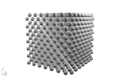
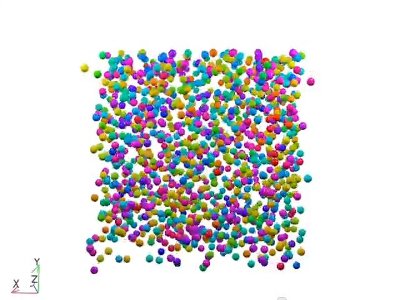
The starting configuration of 1372 hard-spheres with periodic boundary conditions.
DynamO configuration files are XML files. XML files can be opened and edited by your favourite text editor or opened in read only format by any web browser. If you click this link for the example output you will see that web browsers will present the contents of an XML file nicely, but to edit it you will need to save it and open the file again inside a text editor (see the FAQ for more information).
If you open the XML file, config.start.xml, which was generated by dynamod and take a look at the top of the file. You'll notice that there is a short line at the top that identifies this file as an XML file:
<?xml version="1.0"?>Underneath this lies the contents of the file. You will notice that the whole content of the file is enclosed within a pair of DynamOconfig tags. In XML, these are called the root tags:
<DynamOconfig version="1.5.0">...</DynamOconfig>
Whenever some content has been omitted we will try to use "..." to indicate that there is some XML data which we have skipped. There is a version attribute in the DynamOconfig tag which is used by DynamO to warn if the file format is out of date version while loading it. This version number is only incremented when a major change in the file format happens.
Inside the root tags, are several other tags corresponding to different parts of the configuration:
<DynamOconfig version="1.5.0">
  <Simulation lastMFT="0">...</Simulation>
  <Properties/>
  <ParticleData>...</ParticleData>
</DynamOconfig>
The Simulation tags at the top of the file contain the majority of the settings of the simulation, such as the boundary conditions and interactions. Underneath the Simulation tags lies the Properties tag. You can see that the Properties tag is empty in this configuration as it is only needed in polydisperse systems where there are a large number of parameters to set for each particle. The use of properties will be covered in a later tutorial, but for now we can ignore them.
The last set of tags are the ParticleData tag which contains all of the individual particle's data and is the first section discussed in detail.
Underneath the Properties tag, at the bottom of the file, lies the ParticleData tags. You should see lots of Pt tags stored inside the ParticleData tags, like so:
<DynamOconfig>
  <ParticleData>
    <Pt ID="0">
      <P x="-6.4999999999999991" y="-6.4999999999999991" z="-6.4999999999999991"/>
      <V x="-1.8993855827063624" y="-0.7615273462831198" z="-0.46987054041780463"/>
    </Pt>
    <Pt ID="1">
      <P x="-5.4999999999999991" y="-5.4999999999999991" z="-6.4999999999999991"/>
      <V x="0.77139338649244393" y="0.54656534098888188" z="-1.7296148288342952"/>
    </Pt>
    ...
  </ParticleData>
</DynamOconfig>
Each of these Pt tags represent the data of a single particle. Each Pt tag has an ID attribute, which is a unique number used to help you identify the particle. This ID number is not read by DynamO when it loads the configuration file. DynamO currently loads and assigns ID's to the particles in the order they appear in the configuration file. The ID is only written there for your reference of the ID numbers DynamO used in the simulation that produced this file. This may have to change in the future if DynamO ever supports particle insertion and deletion, but for now this makes it very convenient to merge or delete particles in simple systems.
Inside each particle (Pt) tag there are two enclosed tags called P and V. The P tag holds the position of a particle within the system and the V tag holds the particles velocity. You'll notice that DynamO sometimes outputs numerical values in scientific notation to ensure that no precision is lost when loading and saving configurations. For more information on the Pt tag, please see the reference:
You should notice that the mass and size of the particles is not specified here where you might expect it. This is because of the general and unique functional definition of "properties" of particles in DynamO. The problems they address are:
Instead, in DynamO the properties of particles are defined where they are needed and you can map one single value of a property onto a range of particles. For example, if you use a hard sphere Interaction, its inside the corresponding Interaction tag where you have to specify the diameter of the particle. The mass of a particle is defined when you specify the Species of the particles. All of these tags are inside the Simulation tags and are discussed in detail in the following sections.
The Simulation tags are where the details of the system dynamics are stored. There are a huge number of settings that can be adjusted here, so we will deal with each tag separately.
The first tags in the Simulation section of the configuration file are the Scheduler tags.
<DynamOconfig>
  <Simulation>
    <Scheduler Type="NeighbourList">
      <Sorter Type="BoundedPQMinMax3"/>
    </Scheduler>
  </Simulation>
</DynamOconfig>
The Scheduler tags contain the settings for the event Scheduler and the event Sorter, which are the parts of DynamO responsible for determining which event happens next in the simulation. Changing the Scheduler settings should never affect the results DynamO generates. However, optimal settings will greatly increase DynamO's calculation speed. The Scheduler tags will almost always look as they do above, as these are the optimal settings for most simple systems. These settings are to use a neighbour list to detect events, and to use a Bounded Priority Queue on three-element Min-Max heaps for event sorting.
Instead of the "NeighbourList" Type of Scheduler, we could instead use the "Dumb" Type. The Dumb scheduler is the simplest type of Scheduler as it doesn't use a neighbour list but simply tests all pairs of particles for events. This approach is very slow and it is only practical when developing new types of Interactions, or tracking down errors in the Neighbour List implementation. If you try changing the Scheduler type to Dumb in this example configuration you will notice the simulator processes around $1/25^{th}$ of the events per second when compared against the NeighbourList scheduler.
For more information on the Scheduler or Sorter tags and the available Types, please see the reference:
In the Simulation tag there is a tag called SimulationSize which holds the size of the primary simulation domain.
<DynamOconfig>
  <Simulation>
    <SimulationSize x="13.999999999999998" y="13.999999999999998" z="13.999999999999998"/>
  </Simulation>
</DynamOconfig>
The effect of expanding the simulation domain.
Here we can see the simulation is performed in a $14\times14\times14$ domain. We will see in a moment that this system actually has periodic boundary conditions; however, even truely infinite (non-periodic) systems must have some finite size specified for the primary image for the neighbourlist to function, so you always need a SimulationSize tag in your configurations.
If we increase the size of the simulation domain to a $30\times30\times30$ domain, we lower the density of the configuration and produce the video to the right. You should notice that the particles start in the center of the domain and expand outwards to fill the primary image. When using periodic boundary conditions, the positions in the configuration file are always written out in the range $(\pm L_x/2, \pm L_y/2, \pm L_z/2)$ so that the point $(0,0,0)$ lies in the middle of the simulation domain.
If, instead of expanding, we tried to reduce the simulation domain we might find that we run into difficulties. This is because any particles now outside the new, smaller, primary image will be "folded" back into it, possibly causing overlapping particles. With periodic boundary conditions, reducing the size of the simulation is not straightforward and we will have to look at more advanced techniques such as compression if we want to increase a configuration's density.
For more information on the SimulationSize tag, please see the reference:
We will now look into how we can disable this periodic "folding" completely in the following section on boundary conditions.

The same configuration as in the movie above, but with the Boundary Conditions set to None.
Another mandatory tag within the Simulation tags is the Boundary Condition (BC) tag.
<DynamOconfig>
  <Simulation>
    <BC Type="PBC"/>
  </Simulation>
</DynamOconfig>
Here we can see that the current BCs are Periodic Boundary Conditions (PBC). This explains the "popping" of particles near the edges of the simulation in the videos above, as particles are popping from one side of the simulation to the other. If you change the boundary condition type attribute to None, the system will now be an infinite domain without boundaries. The particles will be allowed to fly off in all directions without constraint (see the video on the right), which is very useful if you want to simulate a single isolated polymer, or any system with gravity.
But be warned, if you now try to convert back to periodic boundary conditions by changing the boundary condition type back to PBC, all particle positions will be "folded" back into the primary simulation domain specified by the SimulationSize tag (a cubic $14\times14\times14$ volume). This "folding" will probably result in overlapping particles, so you need to be careful when changing Boundary Conditions from None back to PBC.
There are also Lees-Edwards shearing boundary conditions available in DynamO (Type="LE") which will be discussed in a later tutorial. For more information on the BC tag and the available Types, please see the reference:
The next set of tags in the Simulation section are the Species tags, which are defined within the Genus tags.
<DynamOconfig>
  <Simulation>
    <Genus>
      <Species Mass="1" Name="Bulk" Type="Point">
        <IDRange Type="All"/>
      </Species>
    </Genus>
  </Simulation>
</DynamOconfig>
A single Species tag defines the mass and inertia tensor of a collection of particles. These are unique properties of the particle; therefore, each particle must belong to exactly one species.
The obvious attributes of the Species tag are the Mass of the particles and the Name of the Species. Names are used to identify particles when reporting species-specific results, such as diffusion coefficients, radial distribution functions, and so on.
The Type parameter specifies the class of inertia tensor that the particle has. A value of Point implies that this particle has no rotational degrees of freedom, such as atoms in molecular systems. Other values, such as spherical top or a full tensor are available and are useful when studying granular systems, or assymetric particles. For more information on the Species tag and the available Types, please see the reference:
Inside of the Species tag, there is an IDRange tag which is used to specify which particles this species applies to. IDRanges are discussed in the following section.
The IDRange tags are the most unique (and perhaps confusing) part of the DynamO file format. However, they are a extremely powerful method for mapping properties onto particles.
"Traditionally" in other particle simulators, each particle has its own section of the configuration file (and memory) to store properties such as its mass, diameter, type and so on. Unfortunately, in many simulations many particles have the same properties and this redundant storage of information wastes memory and speed.
What we want is a "functional" definition of properties where we can input statements like "all particles have a mass of 1" . We would like to be able to specify a property once, and then map this property onto a range of particles (see image below).
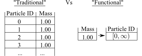
A graphic comparing the traditional method of storing particle data, and the functional method
This "functional" mapping saves memory and the small computational cost of using these definitions is nothing compared to the speed increases due to the reduced use of the memory bandwidth and cache.
But how does this work in DynamO? You might have guessed by now, the range of particle ID's that a property such as the Species maps on to is specified by the IDRange tags. If we take a look at the example configuration file again:
<DynamOconfig>
  <Simulation>
    <Genus>
      <Species Mass="1" Name="Bulk" Type="Point">
        <IDRange Type="All"/>
      </Species>
    </Genus>
  </Simulation>
</DynamOconfig>
Here it is clear to see that the IDRange tag has a Type attribute equal to "All", which means all particles have the same Species (and therefore mass, intertia tensor). Multiple Species can be defined in a straightforward way, and this is discussed in the next tutorial when we consider a binary mixture of spheres. For more information on the IDRange tag and the available Types, please see the reference:
In later tutorials, we will see some more types of IDRanges and how they can be used. We will also see what to do when functional definitions are difficult, such as in polydisperse systems where every particle has a unique mass and size.
The next important tags in the file format are the Interaction tags. These tags are used to specify the interactions between pairs of particles (bonded, non-bonded, whatever). The key definition of an Interaction is an event which involves two-particles. Therefore, every two particle event is specified here, and every pair of particles must have a corresponding Interaction!
If we take a look at the example configuration file again, we have:
<DynamOconfig>
  <Simulation>
    <Interactions>
      <Interaction Type="HardSphere" Diameter="1" Name="Bulk">
        <IDPairRange Type="All"/>
      </Interaction>
    </Interactions>
  </Simulation>
</DynamOconfig>
Here we can see the Type attribute specifying that this is a hard sphere interaction. Hard spheres have a Diameter and Elasticity which are set by the appropriate attributes. All Interactions must have a Name which is used to identify it.
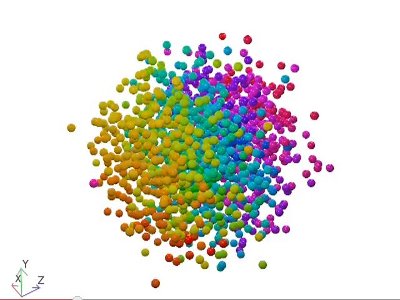
Modifying the Interaction to make a low density granular gas.
We can see the dramatic effect of some simple changes to the Interaction by reducing the particle Diameter to 0.5 and the Elasticity to 0.5. By lowering the Diameter to a half of its previous value, we've reduced the dimensionless density of the system by a factor of $2^3=8$. If you take a look at the video to the right you will see that this density is comparable to the density of the system where we doubled the size of the simulation domain (see the SimulationSize tag above); However, in this case the particles are spread evenly about in space at the start of the simulation. Please note that if you try to increase the Diameter again after running the simulation, you may again cause overlaps!
By lowering the Elasticty, we have also created a granular system. In granular systems, inelastic interactions remove energy over time and the system begins to slow down. You can also see a hint of clustering in the video to the right, which is another characteristic of granular systems.
For more information on the Interaction tag and the available Types, please see the reference:
We have now covered the primary type of events (two particle Interaction events) which will occur in our simulations but there are many other possible event types available. These are grouped into Locals, Globals, and System events, which are discussed below.
There is an IDPairRange tag inside the Interaction tags which is used to specify which particles this interaction applies to. Although IDPairRanges are a similar concept to IDRanges, they are unique in that they specify pairs of particles, not just individual particles. The IDPairRange Type attribute of All specifies all pairs of particles interact this way. IDPairRanges and multiple Interactions are covered in more detail in the next tutorial. A complete description of the IDPairRange tag and all of the available Types is available in the reference:
Enabling gravity causes all the particles to fall, but with periodic boundary conditions there is nothing to arrest their descent.
Finally, the last non-empty tag to discuss is the Dynamics tag:
<DynamOconfig>
  <Simulation>
    <Dynamics Type="Newtonian"/>
  </Simulation>
</DynamOconfig>
The Dynamics tag controls the equations of motion of the system. Any changes you make will alter the fundamental dynamics of the system. For example, you might add a constant downwards force to all particles to mimic the effect of gravity (see right).
<DynamOconfig version="1.5.0">
  <Simulation>
    <Dynamics Type="NewtonianGravity">
      <g x="0" y="-1" z="0"/>
    </Dynamics>
  </Simulation>
</DynamOconfig>
This simulation is not particularly interesting as there are no objects for the particles to fall on to, so the system simply accelerates downwards. We would need to add a wall at the bottom for the particles to collide with to make this more interesting.
By altering the Dynamics tag, you can run compression simulations or use multicanonical potentials to deform the energy landscape of the system. These are relatively advanced topics which will be covered in later tutorials. For more information on the Dynamics tag and the available Types, please see the reference:
In this simple system, there are several unused/empty tags, including the Topology, Locals, Globals, and SystemEvents tags. These are only useful if looking at a more complex systems with polymers, walls, or thermostats. Here, we'll just quickly introduce each tag and link to their configuration reference section.
The Topology tag actually does not affect the dynamics of the system. It is only used as a way to mark out molecules or other multi-particle structures for monitoring and collection of data. For example, you might create a list of the particles in each polymer in your molecular simulation so that you can calculate a molecular (instead of atomic) diffusion coefficient. This tag will become more useful when bonded interactions are introduced in a later tutorial on polymeric systems. For more information on the Topology tag, please see the reference:
A Local is any possible event involving one particle which is localised in space. Typical examples of Locals are are walls, triangle meshes and other fixed objects. The key part of the definition is that the events only occur if the particle is in a certain location in space. This means these events can be optimised by inserting them into a neighbour list.
Globals are single particle events which can occur anywhere (i.e., they cannot be optimised by the use of neighbour lists). A typical example of a Global is the Neighbour list, but this is usually hidden by default. Other examples of global events are Single Occupancy cells and boundary condition enforcers.
SystemEvents comprise every other source of events which does not fit into the categories of a Interaction, Local, or Global. These might be thermostats, umbrella potentials, snapshotting, simulation end conditions or temperature rescalers. This configuration has no System events, but we will see the use of thermostats in the next tutorial.
In this lengthy tutorial we've covered the entire configuration file format. Now that we've covered the general workflow of using DynamO in tutorial 2, and all of the terminology and configuration file format in this tutorial, the following tutorials can focus on case studies of certain systems and collecting data, beginning with the multicomponent square-well fluid.
Page last modified: Thursday 29th July 2021