This is a reference for the configuration file format of DynamO. If you are new to DynamO, please see the general introduction to the file format in tutorial 3 first.

In the following sections, all of the available XML tags and attributes of the configuration file are listed and all of the options are detailed for each tag type. Below is a hyperlinked hierarchy of the tags in the configuration file.

General Structure

¹These tags are just containers and do not have any attributes.

Scheduler

The Scheduler specifies how DynamO searches the simulation for events. How the events are actually sorted by the scheduler is specified through the Sorter tag.

Type="Dumb"

Description

The "Dumb" scheduler is the most basic and slowest scheduler available. When particles undergo an event, the Dumb scheduler tests for new events against all other particles in the system (regardless of where they are). This cost scales linearly with the system size ($\mathcal{O}(N)$), resulting in an overall $\mathcal{O}(N^2)$ scaling of the computational cost. This Scheduler type is only provided for debugging and testing purposes.

Example usage

<Scheduler Type="Dumb">
  <Sorter .../>
</Scheduler>

Full Tag, Subtag, and Attribute List

Type (attribute): Must have the value "Dumb" to select this Scheduler type.
Sorter (tag): This tag specifies the type of event sorter used in the Scheduler. See the section on Sorters for more information on this tag.

Type="NeighbourList"

Description

The "NeighbourList" scheduler uses a NeighbourList to optimise the detection of events. When particles undergo an event, the NeighbourList scheduler only tests for new events against nearby particles. This cost is independent of the system size ($\mathcal{O}(1)$), resulting in an overall linear ($\mathcal{O}(N)$) scaling of the computational cost.

Note

The NeighbourList scheduler will automatically add a Global neighbour-list interaction to the system if one has not already been specified. The current default is the Cells type Global.

If you want to specify the neighbour list type or change its parameters, please add a Global with the name attribute set to "SchedulerNBList" to allow the NeighbourList Scheduler to identify it.

Example usage

<Scheduler Type="NeighbourList">
  <Sorter .../>
</Scheduler>

Full Tag, Subtag, and Attribute List

Type (attribute): Must have the value "NeighbourList" to select this Scheduler type.
Sorter (tag): This tag specifies the type of event sorter used in the Scheduler. See the section on Sorters for more information on this tag.

Sorter

The Sorter tag specifies the method DynamO uses to sort events when determining the next event to occur.

Type="CBT"

Description

The "CBT" Sorter uses a STL priority queue for each particle and inserts this into a Complete Binary Tree (CBT) to sort the events. This type of Sorter is very robust to unusual systems (such as systems with zero or one particle) but, as the computational cost scales as $\mathcal{O}(\log_2(N)$ with the system size, it is not the default Sorter used by DynamO.

Example usage

<Sorter Type="CBT"/>

Full Tag, Subtag, and Attribute List

Type (attribute): Must have the value "CBT" to select this Sorter type.

Type="BoundedPQMinMax3"

Description

The "BoundedPQMinMax3" Sorter uses a bounded MinMax heap of size 3 to sort particle events. These particle queues are then presorted using a bounded priority queue. The earliest entry in the bounded priority queue is then sorted using a Complete Binary Tree. In this way, the lazy deletion scheme can be combined with a fixed size event queue and a bounded priority queue to yield a constant ($\mathcal{O}(1)$) scaling of the computational cost with the system size. There are variants of this scheduler with different sizes of the MinMax heaps ranging from 2 to 8 (e.g., "BoundedPQMinMax8" is also available). After many years of testing this has proven to be the fastest and lowest memory event sorter for a range of event-driven particle simulations. In small systems the CBT Sorter is slightly faster and, depending on the system studied, you may find the MinMax heap size might be increased or decreased to increase performance.

Example usage

<Sorter Type="BoundedPQMinMax3"/>

Full Tag, Subtag, and Attribute List

Type (attribute): Must have the value "BoundedPQMinMax3" to select this Sorter type. Other variants from "BoundedPQMinMax2" to "BoundedPQMinMax8" are also available.

SimulationSize

Description

The SimulationSize tag specifies the dimensions of the primary image for periodic boundary conditions. When the system is not periodic, it specifies the size of the tiled neighbourlist (if one is used). If no neighbour list is used in an infinite system, this tag has no effect.

Example usage

This example specifies a $10\times10\times10$ primary image.

<SimulationSize x="10" y="10" z="10"/>

Full Tag, Subtag, and Attribute List

x (attribute): The size in the $x$ dimension.
y (attribute): The size in the $y$ dimension.
z (attribute): The size in the $z$ dimension.

Species

Species are vital tags used to specify the mass and inertia data of a set of particles. They also provide a unique identifier/name for groups of particles as each particle must belong to exactly one species. Many output plugins use the species of a particle to separate results (for example, a radial distribution function will be generated for all pairings of species in the system).

Particles will have rotational degrees of freedom if they have a Species which provides a non-zero inertia tensor (e.g. "SphericalTop"). Other Species types such as "Point" and "FixedCollider" will avoid the computational overhead of tracking the rotation of the particles.

Type="Point"

Description

This Species type corresponds to point mass (zero inertia) particles, but this type is also used in systems where inertial data is unimportant (atomic or frictionless systems). It is the simplest type of Species available.

Example usage

<Species Mass="1" Name="Bulk" Type="Point">
  <IDRange .../>
</Species>

Full Tag, Subtag, and Attribute List

Type (attribute): Must have the value "Point" to select this Species type.
Mass (attribute): The mass of the particles represented by this Species.
This attribute is a Property specifier with units of Mass (see the section on Properties for more information).
Name (attribute): The name of the particles represented by this Species. This is used in output, so species "A" or "Carbon" are examples. If the system is monocomponent, dynamod often uses the name "Bulk".
IDRange (tag): A IDRange which specifies the Particles represented by this Species tag. The IDRanges of each Species must not overlap with any other Species in the system. All particles must belong to exactly one Species.

Type="FixedCollider"

Description

This Species type corresponds to particles which have infinite mass and no inertia tensor. This is useful for particles which are used as the boundaries of a system (also called a particle mesh).

Example usage

<Species Name="Bulk" Type="FixedCollider">
  <IDRange .../>
</Species>

Full Tag, Subtag, and Attribute List

Type (attribute): Must have the value "FixedCollider" to select this Species type.
Name (attribute): The name of the particles represented by this Species. This is used in output, so species "A" or "Carbon" are examples. If the system is monocomponent, dynamod often uses the name "Bulk".
IDRange (tag): A IDRange which specifies the Particles represented by this Species tag. The IDRanges of each Species must not overlap with any other Species in the system. All particles must belong to exactly one Species.

Type="SphericalTop"

Description

This Species type corresponds to particles where the three principal momenta of inertia are identical. It is also used in systems where only two of the principal momenta of inertia are equal but the rotation is constrained such that the particle cannot precess.

Example usage

<Species Mass="1" Name="Bulk" Type="SphericalTop" InertiaConstant="0.1">
  <IDRange .../>
</Species>

Full Tag, Subtag, and Attribute List

Type (attribute): Must have the value "SphericalTop" to select this Species type.
Mass (attribute): The mass of the particles represented by this Species.
This attribute is a Property specifier with units of Mass (see the section on Properties for more information).
InertiaConstant (attribute): The area factor of the principal momenta of inertia of the particles represented by this Species. This is value is multiplied by the mass of the particle to obtain the value of the principal momenta of inertia.For a solid sphere this value should be $\sigma^2/10$ where $\sigma$ is the particle diameter. A list of inertia constants is available at wikipedia.
Name (attribute): The name of the particles represented by this Species. This is used in output, so species "A" or "Carbon" are examples. If the system is monocomponent, dynamod often uses the name "Bulk".
IDRange (tag): A IDRange which specifies the Particles represented by this Species tag. The IDRanges of each Species must not overlap with any other Species in the system. All particles must belong to exactly one Species.

BC (Boundary Conditions)

The BC tag in the configuration file controls the boundary conditions of the simulation.

Type="None"

Description

The "None" boundary condition actually corresponds to an infinite system, without boundaries. The positions of the particles are not restricted in any dimension.

Example usage

<BC Type="None"/>

Full Tag, Subtag, and Attribute List

Type (attribute): Must have the value "None" to select this BC type.

Type="PBC"

Description

The "PBC" boundary condition applies periodic boundary conditions to every dimension. The positions of the particles are wrapped to fit within the primary image, whose dimensions are specified by the SimulationSize tag.

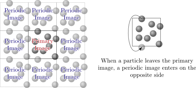
When we want to study molecular fluids we often want the "bulk" properties of the fluid. Effects like surface tension will have a strong influence if there are any free surfaces or boundaries in contact with the fluid, as systems simulated are usually relatively small ($\approx10^5$ molecules). On the other hand, there must be some boundary used to contain the fluid, as using an open (infinite size) system will cause the fluid to either evaporate or form droplets, again with surface effects. To avoid the effects of boundaries/walls while still "containing" the system, periodic boundary conditions are often used. With periodic boundaries, a small representative amount of fluid, called the "primary image," is simulated. This primary image is then surrounded with periodic images which are copies of the primary image as illustrated in the figure below:

An illustration of periodic boundary conditions and the effective wraparound of particle positions.

These boundaries allow the approximation of an infinite fluid using a small repeating image. This is an approximation as the periodicity adds additional correlations to the system, but it is a convenient technique to avoid using real boundaries such as walls to contain the system. When using periodic boundary conditions it is still possible to enter into two-phases if the simulation has attractive interactions, so care must still be taken.

Example usage

<BC Type="PBC"/>

Full Tag, Subtag, and Attribute List

Type (attribute): Must have the value "PBC" to select this BC type.

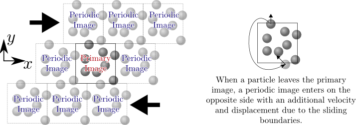
Type="LE"

Description

The "LE" boundary condition applies Lees-Edwards boundary conditions to the system. These are periodic boundary conditions but they shear the system by setting the periodic images in the $y$ direction in motion in the $x$ direction (see figure below). They are also known as sliding-brick boundary conditions.

An illustration of the Lees-Edward sliding-brick boundary condition

Example usage

<BC Type="LE" DXD="0" Rate="1"/>

Full Tag, Subtag, and Attribute List

Type (attribute): Must have the value "LE" to select this BC type.
DXD (attribute): This attribute stores the current displacement of the nearest periodic images in the $x$-direction (units of length).
Rate (attribute): This specifies how fast the boundary is shearing (units of primary image length per unit time).

Structure

Structure tags are used to specify multi-particle structures, such as molecules. This is to mark these structures to allow specialized data collection and to simplify the implementation of complex interactions.

Each Structure tag contains one or more IDRange tags, each of which specifies a single structure of the same type. So one Structure tag has at least the following basic format:

<Topology ...>
  <Structure ...>
    <IDRange .../>
    <IDRange .../>
    ...
  </Structure>
</Topology>

Type="Chain"

Description

The "Chain" Structure is used to mark out a single linear chain molecule.

Example usage

<Structure Type="Chain" Name="Polymer">
  <IDPairRange .../>
</Interaction>

Full Tag, Subtag, and Attribute List

Type (attribute): Must have the value "Chain" to select this Interaction type.
Name (attribute): The name of the Structure. This name is used to identify the Structure in the output generated by the dynarun command. Each Structure should have a name which is unique.
IDRange (tag): This IDRange tag specifies the particles which belong to the linear chain. See the section on IDRange tags for more information on the format of this tag.

Interaction

Interaction tags are used to specify how pairs of particles interact and generate Interaction events.

Each pair of Particle ID's must have a corresponding Interaction.
Every possible pairing of particles (including self pairings) must have a corresponding Interaction, even if they don't interact. If you don't want them to interact at all, you must use a Null Interaction.

The order in which Interactions are listed in the configuration file is important.
When DynamO tests for interactions/events between a pair of particles, it moves through the list of interactions in the order in which they are specified, testing if the ID's of the pair match the Interaction's IDPairRange. Interactions which are higher in the configuration file will override matching Interactions which are lower down.

Each particle must also have a self-Interaction.
This self-Interaction does not generate events, but is used to decide how to draw the particle in the visualiser and to calculate some single particle properties, such as the excluded volume.

Type="Null"

Description

The "Null" Interaction is used to mark particle pairs out as non-interacting. All particle pairs must have a corresponding Interaction defined, so this Interaction is the only way to prevent events being generated for a set of particle pairs.

Example usage

<Interaction Type="Null" Name="Bulk">
  <IDPairRange .../>
</Interaction>

Full Tag, Subtag, and Attribute List

Type (attribute): Must have the value "Null" to select this Interaction type.
Name (attribute): The name of the Interaction. This name is used to identify the Interaction in the configuration file (e.g., see Species) and in the output generated by the dynarun command. Each Interaction must have a name which is unique.
IDPairRange (tag): This IDPairRange tag specifies the pairs of particles which interact using this Interaction. See the section on IDPairRanges for more information on the format of this tag.

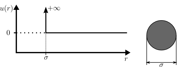
Type="HardSphere"

Description

The "HardSphere" Interaction implements the hard-sphere interaction potential. This is one of the simplest event-driven potentials available.

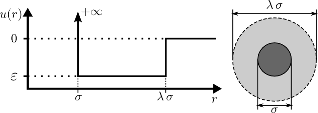
A hard sphere is a simple molecular model used to capture the fundamental effects of "excluded-volume" interactions. You may think of the hard-sphere fluid as an extension of the ideal-gas model, where each molecule now has a diameter, $\sigma$, and cannot overlap the volume of this diameter with the volume of other molecules. The parameters of this model are illustrated below:

The interparticle potential energy of a hard-sphere molecule.

where $u(r)$ is the interparticle potential (which is the potential energy between two particles separated by a distance of $r$). Particles do not interact at separations greater than the diameter of the molecule ($u(r)=0$ for $r\in[\sigma,\,\infty]$). The infinite interaction energy of the hard core ($u(r)=+\infty$ for $r\in[0,\,\sigma]$) makes it energetically impossible for particles to "overlap", therefore the particles will elastically bounce-off of each other when they come into contact.

The effects of this additional "excluded volume" interaction is dramatic and leads to complex transport coefficients as a function of density and the appearance of a fluid-solid freezing transition. This model is too simple to capture any complex temperature effects, such as a liquid/gas phase transition, as it has no finite interaction energies (unlike the square-well fluid). Despite its simplicity, the structure of many real crystals is dominated by the repulsive "excluded-volume" interactions caused by overlapping electron clouds which may be effectively captured by the hard-sphere model. It is also at the heart of kinetic theory which is the most successful attempt to predict the transport properties of fluids from their molecular interactions. The interparticle potential of this model is given in the figure below:

Collision rule

To perform an interaction we need a collision rule which calculates the post-collision velocities of the two particles undergoing the Interaction. The collision rule expresses the post-collision velocities in terms of the pre-collision values.

Show/hide derivation of collision rule

Using the definition of the relative velocity $\boldsymbol{v}_{ij}=\boldsymbol{v}_{i}-\boldsymbol{v}_{j}$ of two particles $i$ and $j$, and the identities $\boldsymbol{v}_i=\boldsymbol{v}_{ij}+\boldsymbol{v}_j$ and $\boldsymbol{v}_j=\boldsymbol{v}_i-\boldsymbol{v}_{ij}$, we have \[\begin{align} \boldsymbol{v}_j'-\boldsymbol{v}_j&=\boldsymbol{v}_i'-\boldsymbol{v}_i - \boldsymbol{v}_{ij}'+\boldsymbol{v}_{ij} \end{align}\] where the primes denote post-collision values. Using the conservation of momentum, we can write \[\begin{align} m_i\,\boldsymbol{v}_i'+m_j\,\boldsymbol{v}_j'&=m_i\,\boldsymbol{v}_i+m_j\,\boldsymbol{v}_j\\ \boldsymbol{v}_i'-\boldsymbol{v}_i&=-\frac{m_j}{m_i}\left(\boldsymbol{v}_j'-\boldsymbol{v}_j\right) \end{align}\] where $m_i$ is the mass of particle $i$. Using the equation derived from the conservation of momentum to eliminate $\boldsymbol{v}_j$ terms, we have \[\begin{align} \boldsymbol{v}_i'-\boldsymbol{v}_i&=-\frac{m_j}{m_i}\left(\boldsymbol{v}_i'-\boldsymbol{v}_i - \boldsymbol{v}_{ij}'+\boldsymbol{v}_{ij}\right)\\ &=m_i^{-1}\,\mu\left(\boldsymbol{v}_{ij}'-\boldsymbol{v}_{ij}\right) \end{align}\] where $\mu_{ij}=\left(m_i^{-1}+m_j^{-1}\right)^{-1}$ is the reduced mass. Therefore we can calculate the post-collision velocities of the particles if we know the change in the relative velocities. For smooth particles the velocities only change along the line of contact, and we have: \[\begin{align*} \left[\boldsymbol{v}_{ij}'\right]_\parallel&=-\varepsilon\left[\boldsymbol{v}_{ij}\right]_\parallel & \left[\boldsymbol{v}_{ij}'\right]_\perp&=\left[\boldsymbol{v}_{ij}\right]_\perp \end{align*}\] where $\varepsilon$ is the elasticity/coefficient of restitution and the subscript $\parallel$ and $\perp$ denote the components parallel and perpendicular to the line of contact. These are calculated like so $\boldsymbol{v}_{ij,\parallel}=\hat{\boldsymbol{r}}_{ij}\left(\hat{\boldsymbol{r}}_{ij}\cdot\boldsymbol{v}_{ij}\right)$ and $\boldsymbol{v}_{ij,\perp}=-\hat{\boldsymbol{r}}_{ij}\times\left(\hat{\boldsymbol{r}}_{ij}\times\boldsymbol{v}_{ij}\right)$ where $\hat{\boldsymbol{r}}_{ij}$ is the unit vector in the direction of the relative separation at contact, $\boldsymbol{r}_{ij}=\boldsymbol{r}_i-\boldsymbol{r}_j$, and $\boldsymbol{r}_i$ is the position of particle $i$. Combining these rules results in the following expression \[\begin{align*} \boldsymbol{v}_{ij}'-\boldsymbol{v}_{ij}=-(1+\varepsilon)\left(\hat{\boldsymbol{r}}_{ij}\cdot\boldsymbol{v}_{ij}\right)\hat{\boldsymbol{r}}_{ij} \end{align*}\] This leads to the final expressions for smooth particles: \[\begin{align} \boldsymbol{v}_i'-\boldsymbol{v}_i&=-m_i^{-1}\,\mu_{ij}(1+\varepsilon)\left(\hat{\boldsymbol{r}}_{ij}\cdot\boldsymbol{v}_{ij}\right)\hat{\boldsymbol{r}}_{ij}\\ \boldsymbol{v}_j'-\boldsymbol{v}_j&=+m_j^{-1}\,\mu_{ij}(1+\varepsilon)\left(\hat{\boldsymbol{r}}_{ij}\cdot\boldsymbol{v}_{ij}\right)\hat{\boldsymbol{r}}_{ij} \end{align}\] In rough systems, particles will change rotation due to interactions. To define the dynamics in such a system we need to consider the relative surface velocity at the point of contact, $\boldsymbol{g}_{ij}$, calculated as follows \[\begin{align*} \boldsymbol{g}_{ij}&=\left(\boldsymbol{v}_i-\boldsymbol{\omega}_i\times R_i\,\hat{\boldsymbol{r}}_{ij}\right)-\left(\boldsymbol{v}_j+\boldsymbol{\omega}_j\times R_j\hat{\boldsymbol{r}}_{ij}\right)\\ &=\boldsymbol{v}_{ij}-\left(R_i\,\boldsymbol{\omega}_i+R_j\,\boldsymbol{\omega}_j\right)\times\hat{\boldsymbol{r}}_{ij} \end{align*}\] where $\boldsymbol{\omega}_j$ is the angular velocity and $R_i$ is the radus of particle $i$. In this case, we can define a normal and a tangential coefficient of restitution as follows \[\begin{align} \left[\boldsymbol{g}_{ij}\right]_\parallel'&=-\varepsilon^n\left[\boldsymbol{g}_{ij}\right]_\parallel & \left[\boldsymbol{g}_{ij}\right]_\perp'&=\varepsilon^t\left[\boldsymbol{g}_{ij}\right]_\perp \end{align}\] where $\boldsymbol{g}_{ij,\parallel}=\hat{\boldsymbol{r}}_{ij}\left(\hat{\boldsymbol{r}}_{ij}\cdot\boldsymbol{g}_{ij}\right)$ and $\boldsymbol{g}_{ij,\perp}=-\hat{\boldsymbol{r}}_{ij}\times\left(\hat{\boldsymbol{r}}_{ij}\times\boldsymbol{g}_{ij}\right)$. Noting that $\boldsymbol{x}=\hat{\boldsymbol{e}}(\hat{\boldsymbol{e}}\cdot\boldsymbol{x})-\hat{\boldsymbol{e}}\times\left(\hat{\boldsymbol{e}}\times\boldsymbol{x}\right)$, these definitions lead to the following expressions \[\begin{align*} \hat{\boldsymbol{r}}_{ij}\left(\hat{\boldsymbol{r}}_{ij}\cdot\left[\boldsymbol{g}_{ij}'-\boldsymbol{g}_{ij}\right]\right)&=-(1+\varepsilon^n)\hat{\boldsymbol{r}}_{ij}\left(\hat{\boldsymbol{r}}_{ij}\cdot\boldsymbol{g}_{ij}\right) & \hat{\boldsymbol{r}}_{ij}\times\left(\hat{\boldsymbol{r}}_{ij}\times\left[\boldsymbol{g}_{ij}'-\boldsymbol{g}_{ij}\right]\right)&=(\varepsilon^t-1)\hat{\boldsymbol{r}}_{ij}\times\left(\hat{\boldsymbol{r}}_{ij}\times\boldsymbol{g}_{ij}\right) \end{align*}\] We need to find an expression which closes the linear momentum balance by providing a relationship between $\boldsymbol{v}_{ij}'-\boldsymbol{v}_{ij}$ and $\boldsymbol{g}_{ij}'-\boldsymbol{g}_{ij}$, as well as determining how the angular velocity changes. Beginning with the angular velocity, we take the contact point as the origin about which the angular momentum is defined. We then note that all contact forces act through the origin and see that angular velocity is conserved for both particles separately. Thus we will have two separate angular-momentum conservation rules: \[\begin{align*} m_i\,R_i\,\hat{\boldsymbol{r}}_{ij}\times\boldsymbol{v}_i' + \boldsymbol{I}_i\cdot\boldsymbol{\omega}_i' &= m_i\,R_i\,\hat{\boldsymbol{r}}_{ij}\times\boldsymbol{v}_i + \boldsymbol{I}_i\cdot\boldsymbol{\omega}_i\\ m_j\,R_j\,\hat{\boldsymbol{r}}_{ij}\times\boldsymbol{v}_j' - \boldsymbol{I}_j\cdot\boldsymbol{\omega}_j' &= m_j\,R_j\,\hat{\boldsymbol{r}}_{ij}\times\boldsymbol{v}_j - \boldsymbol{I}_j\cdot\boldsymbol{\omega}_j \end{align*}\] For symmetric objects we have an isotropic inertia tensor $\boldsymbol{I}_i=I_i\,\boldsymbol{1}$, and can define a reduced moment of inertia as $\tilde{I}_i=I_i/m_i\,R_i^2$ and can rearrange these two equations like so \[\begin{align*} \boldsymbol{\omega}_i'- \boldsymbol{\omega}_i&=- R_i^{-1}\tilde{I}_i^{-1}\left[\hat{\boldsymbol{r}}_{ij}\times\left(\boldsymbol{v}_i' -\boldsymbol{v}_i\right)\right]\\ \boldsymbol{\omega}_j'- \boldsymbol{\omega}_j &= + R_j^{-1}\tilde{I}_j^{-1}\left[\hat{\boldsymbol{r}}_{ij}\times\left(\boldsymbol{v}_j' -\boldsymbol{v}_j\right)\right] \end{align*}\] We need to find the post-collision linear velocities to close these expressions. We can define the pre and post collision relative velocity at the surface as follows \[\begin{align*} \boldsymbol{g}_{ij}&=\left(\boldsymbol{v}_i-\boldsymbol{\omega}_i\times R_i\,\hat{\boldsymbol{r}}_{ij}\right)-\left(\boldsymbol{v}_j+\boldsymbol{\omega}_j\times R_j\hat{\boldsymbol{r}}_{ij}\right)\\ &=\boldsymbol{v}_{ij}-\left(R_i\,\boldsymbol{\omega}_i+R_j\,\boldsymbol{\omega}_j\right)\times\hat{\boldsymbol{r}}_{ij} \end{align*}\] Finding the post collision value of this \[\begin{align*} \boldsymbol{g}_{ij}'&=\boldsymbol{v}_{ij}'-\left(R_i\,\boldsymbol{\omega}_i'+R_j\,\boldsymbol{\omega}_j'\right)\times\hat{\boldsymbol{r}}_{ij}\\ &=\boldsymbol{v}_{ij}' - \left(R_i\left(\boldsymbol{\omega}_i - R_i^{-1}\,\tilde{I}_i^{-1}\left[\hat{\boldsymbol{r}}_{ij}\times\left(\boldsymbol{v}_i' -\boldsymbol{v}_i\right)\right]\right)+R_j\left(\boldsymbol{\omega}_j + R_j^{-1}\,\tilde{I}_j^{-1}\left[\hat{\boldsymbol{r}}_{ij}\times\left(\boldsymbol{v}_j' -\boldsymbol{v}_j\right)\right]\right)\right)\times\hat{\boldsymbol{r}}_{ij}\\ &=\boldsymbol{v}_{ij}'-\left(R_i\,\boldsymbol{\omega}_i + R_j\,\boldsymbol{\omega}_j\right)\times\hat{\boldsymbol{r}}_{ij} + \left(\tilde{I}_i^{-1}\left[\hat{\boldsymbol{r}}_{ij}\times\left(\boldsymbol{v}_i' -\boldsymbol{v}_i\right)\right] -\tilde{I}_j^{-1}\left[\hat{\boldsymbol{r}}_{ij}\times\left(\boldsymbol{v}_j' -\boldsymbol{v}_j\right)\right]\right)\times\hat{\boldsymbol{r}}_{ij} \end{align*}\] Subtracting the pre-collision value from this value, and assuming that all particles have the same reduced moment of inertia, we have \[\begin{align*} \boldsymbol{g}_{ij}'-\boldsymbol{g}_{ij}&=\boldsymbol{v}_{ij}'-\boldsymbol{v}_{ij}+ \tilde{I}^{-1}\left(\left[\hat{\boldsymbol{r}}_{ij}\times\left(\boldsymbol{v}_i' -\boldsymbol{v}_i\right)\right] -\left[\hat{\boldsymbol{r}}_{ij}\times\left(\boldsymbol{v}_j' -\boldsymbol{v}_j\right)\right]\right)\times\hat{\boldsymbol{r}}_{ij}\\ &=\boldsymbol{v}_{ij}'-\boldsymbol{v}_{ij}- \tilde{I}^{-1}\,\hat{\boldsymbol{r}}_{ij}\times\left[\hat{\boldsymbol{r}}_{ij}\times\left(\boldsymbol{v}_{ij}' -\boldsymbol{v}_{ij}\right)\right] \end{align*}\] Now that we have the relationship between $\boldsymbol{g}_{ij}'-\boldsymbol{g}_{ij}$ and $\boldsymbol{v}_{ij}'-\boldsymbol{v}_{ij}$, we look to insert the coefficients of restitution. We notice that the second term is perpendicular to $\hat{\boldsymbol{r}}_{ij}$, therefore we have \[\begin{align} \hat{\boldsymbol{r}}_{ij}\cdot\left(\boldsymbol{v}_{ij}'-\boldsymbol{v}_{ij}\right) = \hat{\boldsymbol{r}}_{ij}\cdot\left(\boldsymbol{g}_{ij}'-\boldsymbol{g}_{ij}\right) \end{align}\] Taking the vector product instead and we have \[\begin{align*} \hat{\boldsymbol{r}}_{ij}\times\left[\boldsymbol{g}_{ij}'-\boldsymbol{g}_{ij}\right] &=\hat{\boldsymbol{r}}_{ij}\times\left[\boldsymbol{v}_{ij}'-\boldsymbol{v}_{ij}\right]- \tilde{I}^{-1}\hat{\boldsymbol{r}}_{ij}\times\left[\hat{\boldsymbol{r}}_{ij}\times\left[\hat{\boldsymbol{r}}_{ij}\times\left(\boldsymbol{v}_{ij}' -\boldsymbol{v}_{ij}\right)\right]\right] \end{align*}\] we note that $\hat{\boldsymbol{e}}\times\left(\hat{\boldsymbol{e}}\times\left(\hat{\boldsymbol{e}}\times\boldsymbol{x}\right)\right)=-\hat{\boldsymbol{e}}\times\boldsymbol{x}$, giving \[\begin{align} \hat{\boldsymbol{r}}_{ij}\times\left[\boldsymbol{g}_{ij}'-\boldsymbol{g}_{ij}\right] &=\hat{\boldsymbol{r}}_{ij}\times\left[\boldsymbol{v}_{ij}'-\boldsymbol{v}_{ij}\right]+ \tilde{I}^{-1}\,\hat{\boldsymbol{r}}_{ij}\times\left(\boldsymbol{v}_{ij}' -\boldsymbol{v}_{ij}\right)\nonumber\\ \hat{\boldsymbol{r}}_{ij}\times\left[\boldsymbol{v}_{ij}'-\boldsymbol{v}_{ij}\right]&=\left(1+\tilde{I}^{-1}\right)^{-1}\hat{\boldsymbol{r}}_{ij}\times\left[\boldsymbol{g}_{ij}'-\boldsymbol{g}_{ij}\right] \end{align}\] Noting again that in general we have $\boldsymbol{x}=\hat{\boldsymbol{e}}(\hat{\boldsymbol{e}}\cdot\boldsymbol{x})-\hat{\boldsymbol{e}}\times\left(\hat{\boldsymbol{e}}\times\boldsymbol{x}\right)$, and we can write \[\begin{align} \boldsymbol{v}_{ij}'-\boldsymbol{v}_{ij}&=\hat{\boldsymbol{r}}_{ij}\left(\hat{\boldsymbol{r}}_{ij}\cdot(\boldsymbol{v}_{ij}'-\boldsymbol{v}_{ij})\right) -\hat{\boldsymbol{r}}_{ij}\times\left[\hat{\boldsymbol{r}}_{ij}\times\left(\boldsymbol{v}_{ij}'-\boldsymbol{v}_{ij}\right)\right]\\ &=\hat{\boldsymbol{r}}_{ij}\left(\hat{\boldsymbol{r}}_{ij}\cdot\left(\boldsymbol{g}_{ij}'-\boldsymbol{g}_{ij}\right)\right) -\left(1+\tilde{I}^{-1}\right)^{-1}\hat{\boldsymbol{r}}_{ij}\times\left[\hat{\boldsymbol{r}}_{ij}\times\left[\boldsymbol{g}_{ij}'-\boldsymbol{g}_{ij}\right]\right] \end{align}\] Inserting in the coefficients of restitution, we have \[\begin{align} \boldsymbol{v}_{ij}'-\boldsymbol{v}_{ij}&=-(1+\varepsilon^n)\hat{\boldsymbol{r}}_{ij}\left(\hat{\boldsymbol{r}}_{ij}\cdot\boldsymbol{g}_{ij}\right) -\left(1+\tilde{I}^{-1}\right)^{-1}(\varepsilon^t-1)\hat{\boldsymbol{r}}_{ij}\times\left(\hat{\boldsymbol{r}}_{ij}\times\boldsymbol{g}_{ij}\right) \end{align}\] Using this we can complete the expression for the linear velocity change: \[\begin{align} \boldsymbol{v}_i'-\boldsymbol{v}_i&=-m_i^{-1}\,\mu_{ij}\left((1+\varepsilon^n) \hat{\boldsymbol{r}}_{ij}\left(\hat{\boldsymbol{r}}_{ij}\cdot\boldsymbol{g}_{ij}\right) +\left(1+\tilde{I}^{-1}\right)^{-1}(\varepsilon^t-1) \hat{\boldsymbol{r}}_{ij}\times\left(\hat{\boldsymbol{r}}_{ij}\times\boldsymbol{g}_{ij}\right)\right) \end{align}\] Inserting this into the expression for the change in angular velocity, we have \[\begin{align*} \boldsymbol{\omega}_i'- \boldsymbol{\omega}_i&=- R_i^{-1}\tilde{I}_i^{-1}\left[\hat{\boldsymbol{r}}_{ij}\times\left(\boldsymbol{v}_i' -\boldsymbol{v}_i\right)\right]\\ &= m_i^{-1}\,\mu_{ij}\,R_i^{-1}\left(1+\tilde{I}\right)^{-1}(\varepsilon^t-1)\hat{\boldsymbol{r}}_{ij}\times\left[ \hat{\boldsymbol{r}}_{ij}\times\left(\hat{\boldsymbol{r}}_{ij}\times\boldsymbol{g}_{ij}\right)\right]\\ &= -m_i^{-1}\,\mu_{ij}\,R_i^{-1}\left(1+\tilde{I}\right)^{-1}(\varepsilon^t-1)\hat{\boldsymbol{r}}_{ij}\times\boldsymbol{g}_{ij} \end{align*}\] The corresponding rules for particle $j$ follow with similar reasoning or through relabing and noting that $\boldsymbol{g}_{ji}=-\boldsymbol{g}_{ij}$. In summary, we have

\[\begin{align*} \boldsymbol{v}_i'-\boldsymbol{v}_i&=-\frac{\mu_{ij}}{m_i}\left((1+\varepsilon^n) \hat{\boldsymbol{r}}_{ij}\left(\hat{\boldsymbol{r}}_{ij}\cdot\boldsymbol{g}_{ij}\right) +\frac{\varepsilon^t-1}{1+\tilde{I}^{-1}} \hat{\boldsymbol{r}}_{ij}\times\left(\hat{\boldsymbol{r}}_{ij}\times\boldsymbol{g}_{ij}\right)\right)\\ \boldsymbol{v}_j'-\boldsymbol{v}_j&=\frac{\mu_{ij}}{m_j}\left((1+\varepsilon^n) \hat{\boldsymbol{r}}_{ij}\left(\hat{\boldsymbol{r}}_{ij}\cdot\boldsymbol{g}_{ij}\right) +\frac{\varepsilon^t-1}{1+\tilde{I}^{-1}} \hat{\boldsymbol{r}}_{ij}\times\left(\hat{\boldsymbol{r}}_{ij}\times\boldsymbol{g}_{ij}\right)\right)\\ \boldsymbol{\omega}_i'- \boldsymbol{\omega}_i&=-\frac{\mu_{ij}(\varepsilon^t-1)}{m_i\,R_i\left(1+\tilde{I}\right)} \hat{\boldsymbol{r}}_{ij}\times\boldsymbol{g}_{ij} \\ \boldsymbol{\omega}_j'- \boldsymbol{\omega}_j&=-\frac{\mu_{ij}(\varepsilon^t-1)}{m_j\,R_j\left(1+\tilde{I}\right)}\hat{\boldsymbol{r}}_{ij}\times\boldsymbol{g}_{ij} \end{align*}\] where $\varepsilon^n$ and $\varepsilon^t$ are the normal and tangential coefficient of elasticity respectively. See the derivation above for more information on the symbols and their meaning.

Example usage

<Interaction Type="HardSphere" Diameter="1" Name="Bulk">
  <IDPairRange .../>
</Interaction>

Full Tag, Subtag, and Attribute List

Type (attribute): Must have the value "HardSphere" to select this Interaction type.
Diameter (attribute): The interaction diameter ($\sigma$) of the particle pairs corresponding to this Interaction.
This attribute is a Property specifier with a unit of Length (see the section on Properties for more information).
Elasticity (attribute): This is an optional attribute. The elasticity, $\varepsilon^n$, controls the dissipation of translational energy between interacting particles. This value is typically 1 for molecular systems and between zero and one for granular systems. If the attribute is unset, it is equivalent to Elasticity="1".
This attribute is a Property specifier with Dimensionless units (see the section on Properties for more information).
TangentialElasticity (attribute): This is an optional attribute. The tangential elasticity, $\varepsilon^t$, controls the dissipation/generation of energy between interacting particles in the tangential/rotational direction and is typically in the range $[-1,1]$. If the tangential elasticity is one, there is no tangential interaction, whereas TangentialElasticity="-1" corresponds to a complete reversal of the relative surface velocities. It is important to note that setting the TangentialElasticity attribute requires that the particles have a Species with inertia information. If the attribute is unset then rotational dynamics are ignored and the particles can have any Species type.
This attribute is a Property specifier with Dimensionless units (see the section on Properties for more information).
Name (attribute): The name of the Interaction. This name is used to identify the Interaction in the output generated by the dynarun command. Each Interaction must have a name which is unique.
IDPairRange (tag): This IDPairRange tag specifies the pairs of particles which interact using this Interaction. See the section on IDPairRanges for more information on the format of this tag.

Type="SquareWell"

Description

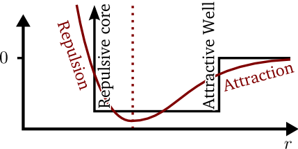
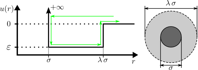
The "SquareWell" Interaction implements the square-well interaction potential, illustrated in the figure below.

A square-well molecule is a particle which has a hard-core diameter of $\sigma$ and is surrounded by an attractive well with a diameter of $\lambda\,\sigma$ and a depth of $\varepsilon$. These variables are illustrated in the diagram below:

A diagram of a square-well molecule including its parameters.

where $u(r)$ is the interparticle potential (which is the potential energy between two particles separated by a distance of $r$).

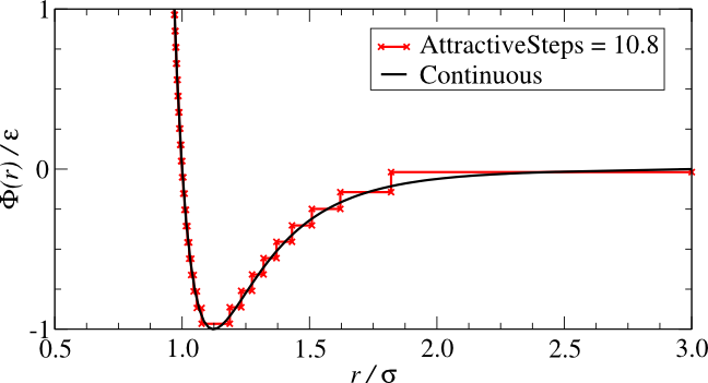
Square-well molecules are simple models which display the two fundamental features of real molecules, a short range repulsion (due to overlapping electron clouds) and longer ranged attraction (due to van-der-waals/London/dispersion forces). A comparison of the square-well model (black) and a "realistic" interatomic potential (red) is given in the figure below:

A comparision of a square-well potential and a "realistic" potential..

It is clear that the square-well potential is a rough approximation of the "realistic" potential, but its dynamics are not immediately clear. With the "realistic" potential, it is easy to see how a pair of particles might "fall down" the potential and attract or repulse each other, but how does this behaviour appear in the square-well model? When two distant square-well particles approach each other and reach a separation of $r=\lambda\,\sigma$, they enter the well (or "capture" each other) and a momentum impulse increases their kinetic energy by $\varepsilon$ (they are attracted to each other). If they then approach the inner core and reach a separation of $r=\sigma$, they will be unable to pay the infinite energy cost to enter the core and will instead elastically bounce off it. Once they begin to retreat from each other (either by bouncing off the core or by missing it) and reach a separation of $r=\lambda\,\sigma$, they must have enough kinetic energy in the direction of the well to escape it and pay the energy cost, $\varepsilon$, otherwise they will bounce off the inside of the well (both are attractive interactions).

If we used more steps to more accurately approximate the "realistic" potential (see the "Stepped" type Interaction), we can quite quickly capture the full behaviour of the smooth/"realistic" potential. However, the square-well model is so interesting because it is so simple! We can make progress in understanding it theoretically and, if we can understand the fundamental behaviour of square-well molecules, the fundamental behaviour of realistic potentials can also be explained.

Example usage

<Interaction Type="SquareWell" Diameter="1" Elasticity="1" Lambda="1.5" WellDepth="1" Name="Bulk">
  <IDPairRange .../>
  <CaptureMap .../>
</Interaction>

Full Tag, Subtag, and Attribute List

Type (attribute): Must have the value "SquareWell" to select this Interaction type.
Diameter (attribute): The interaction diameter ($\sigma$) of the particle pairs corresponding to this Interaction.
This attribute is a Property specifier with a unit of Length (see the section on Properties for more information).
Elasticity (attribute): The elasticity of the particle pairs corresponding to this Interaction. This value is typically 1 for molecular systems and between zero and one for granular systems.
This attribute is a Property specifier with Dimensionless units (see the section on Properties for more information).
Lambda (attribute): The well-width factor ($\lambda$) of the particle pairs corresponding to this Interaction. Values below 1 are not valid.
This attribute is a Property specifier with Dimensionless units (see the section on Properties for more information).
WellDepth (attribute): The interaction energy ($\varepsilon$) of the particle pairs corresponding to this Interaction.
This attribute is a Property specifier with a unit of Energy (see the section on Properties for more information).
Name (attribute): The name of the Interaction. This name is used to identify the Interaction in the output generated by the dynarun command. Each Interaction must have a name which is unique.
CaptureMap (tag): If present, the CaptureMap tag should store the particle pairs which are within the well. If it is not present, it will be automatically generated when the configuration is next loaded by dynarun or dynamod. The data in this tag must be correct at all times otherwise errors in the dynamics will occur so take care when manually editing the configuration file. See the reference entry on CaptureMap for more details.
IDPairRange (tag): This IDPairRange tag specifies the pairs of particles which interact using this Interaction. See the section on IDPairRanges for more information on the format of this tag.

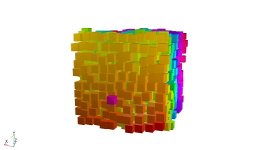
Type="ParallelCubes"

A simulation of Parallel hard cubes.

Description

The "ParallelCubes" Interaction implements the hard cube interaction potential where the cubes do not rotate and are axis-aligned (a video of this system is presented to the right).

Example usage

<Interaction Type="ParallelCubes" Diameter="1" Elasticity="1" Name="Bulk">
  <IDPairRange .../>
</Interaction>

Full Tag, Subtag, and Attribute List

Type (attribute): Must have the value "ParallelCubes" to select this Interaction type.
Diameter (attribute): The interaction diameter is the length at which the particle pairs collide with this Interaction (the length of a cube side).
This attribute is a Property specifier with a unit of Length (see the section on Properties for more information).
Elasticity (attribute): The elasticity of the particle pairs corresponding to this Interaction. This value is typically 1 for molecular systems and between zero and one for granular systems.
This attribute is a Property specifier with Dimensionless units (see the section on Properties for more information).
Name (attribute): The name of the Interaction. This name is used to identify the Interaction in the output generated by the dynarun command. Each Interaction must have a name which is unique.
IDPairRange (tag): This IDPairRange tag specifies the pairs of particles which interact using this Interaction. See the section on IDPairRanges for more information on the format of this tag.

Type="Lines"

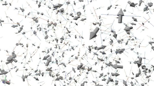
A simulation of Infinitely-thin rods.

Description

The "Lines" Interaction implements the hard infinitely-thin rods interaction potential (a video of this system is presented to the right).

Example usage

<Interaction Type="Lines" Length="1" Elasticity="1" Name="Bulk">
  <IDPairRange .../>
</Interaction>

Full Tag, Subtag, and Attribute List

Type (attribute): Must have the value "Lines" to select this Interaction type.
Length (attribute): The length of the lines.
This attribute is a Property specifier with a unit of Length (see the section on Properties for more information).
Elasticity (attribute): The elasticity of the particle pairs corresponding to this Interaction. This value is typically 1 for molecular systems and between zero and one for granular systems.
This attribute is a Property specifier with Dimensionless units (see the section on Properties for more information).
Name (attribute): The name of the Interaction. This name is used to identify the Interaction in the output generated by the dynarun command. Each Interaction must have a name which is unique.
IDPairRange (tag): This IDPairRange tag specifies the pairs of particles which interact using this Interaction. See the section on IDPairRanges for more information on the format of this tag.

Type="Stepped"

Description

The "Stepped" Interaction wraps a generic spherically-symmetric stepped Potential and uses it for two-particle interactions. This can be used to implement many simple systems (hard-spheres, square-wells) and many complex systems such as a discontinuous Lennard-Jones potential. An alternative approach is to use a "Umbrella" System event to bind collections of particles together using a Potential.

Example usage

Generic wrapping of a Potential.

<Interaction Type="Stepped" Name="Bulk" LengthScale="1" EnergyScale="1">
  <IDPairRange .../>
  <Potential .../>
  <CaptureMap .../>
</Interaction>

Full Tag, Subtag, and Attribute List

Type (attribute): Must have the value "Stepped" to select this Interaction type.
Name (attribute): The name of the Interaction. This name is used to identify the Interaction in the output generated by the dynarun command. Each Interaction must have a name which is unique.
LengthScale (attribute): The length scale by which the Potential is scaled for each particle. For example, if a Lennard-Jones type Potential is used, this sets the $\sigma$ value for each particle.
This attribute is a Property specifier with a unit of Length (see the section on Properties for more information).
EnergyScale (attribute): The energy scale by which the Potential is scaled for each particle. For example, if a Lennard-Jones type Potential is used, this sets the $\varepsilon$ value for each particle.
This attribute is a Property specifier with a unit of Length (see the section on Properties for more information).
Potential (tag): The Potential tag specifies the stepped potential used for this interaction. Please see the section on the Potential tag for more information.
CaptureMap (tag): If present, the CaptureMap tag should store the current step of any particle pairs which are inside the Interaction range of the potential. If it is not present, it will be automatically generated when the configuration is next loaded by dynarun or dynamod. The data in this tag must be correct at all times otherwise errors in the dynamics will occur so take care when manually editing the configuration file. See the reference entry on CaptureMap for more details.
IDPairRange (tag): This IDPairRange tag specifies the pairs of particles which interact using this Interaction. See the section on IDPairRanges for more information on the format of this tag.

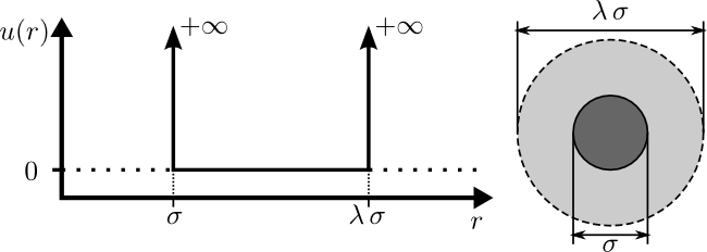
Type="ThinThread"

Description

The "ThinThread" Interaction implements a square-well potential which has hysteresis. The particle behaves as a hard sphere, but once a pair of particles collide with the hard core, they enter the well. The energy of this well must be paid to escape, thus the model loses energy each time particles enter the well. Once particles escape the well, they must again collide with the core before they can re-enter the well (as illustrated in the figure below). This model may be used to model wet granulate and the formation of liquid bridges as when wet granular particles contact each other a liquid bridge stretches between them. Breaking this bridge requires an amount of energy and distance to overcome the surface tension (modelled by the well), but once the bridge is broken the particles will only interact again at short distances.

The interaction potential of a thin thread molecule demonstrating its hysteresis and its parameters

Example usage

<Interaction Type="ThinThread" Diameter="1" Elasticity="1" Lambda="1.5" WellDepth="1" Name="Bulk">
  <IDPairRange .../>
  <CaptureMap .../>
</Interaction>

Full Tag, Subtag, and Attribute List

Type (attribute): Must have the value "ThinThread" to select this Interaction type.
Diameter (attribute): The interaction diameter ($\sigma$) of the particle pairs corresponding to this Interaction.
This attribute is a Property specifier with a unit of Length (see the section on Properties for more information).
Elasticity (attribute): The elasticity of the particle pairs corresponding to this Interaction. This value is typically 1 for molecular systems and between zero and one for granular systems.
This attribute is a Property specifier with Dimensionless units (see the section on Properties for more information).
Lambda (attribute): The well-width factor ($\lambda$) of the particle pairs corresponding to this Interaction. Values below 1 are not valid.
This attribute is a Property specifier with Dimensionless units (see the section on Properties for more information).
WellDepth (attribute): The interaction energy ($\varepsilon$) of the particle pairs corresponding to this Interaction.
This attribute is a Property specifier with a unit of Energy (see the section on Properties for more information).
Name (attribute): The name of the Interaction. This name is used to identify the Interaction in the output generated by the dynarun command. Each Interaction must have a name which is unique.
CaptureMap (tag): If present, the CaptureMap tag should store the particle pairs which are within the well. If it is not present, it will be automatically generated when the configuration is next loaded by dynarun or dynamod. The data in this tag must be correct at all times otherwise errors in the dynamics will occur so take care when manually editing the configuration file. See the reference entry on CaptureMap for more details.
IDPairRange (tag): This IDPairRange tag specifies the pairs of particles which interact using this Interaction. See the section on IDPairRanges for more information on the format of this tag.

Type="SquareBond"

Description

The "SquareBond" Interaction implements a square-well potential with an infinite interaction energy. This allows you to bond particles together to form polymeric structures.

The square-bond interaction potential and its parameters.

Example usage

<Interaction Type="SquareBond" Diameter="1" Elasticity="1" Lambda="1.5" Name="Bulk">
  <IDPairRange .../>
</Interaction>

Full Tag, Subtag, and Attribute List

Type (attribute): Must have the value "SquareBond" to select this Interaction type.
Diameter (attribute): The interaction diameter ($\sigma$) of the particle pairs corresponding to this Interaction.
This attribute is a Property specifier with a unit of Length (see the section on Properties for more information).
Elasticity (attribute): The elasticity of the particle pairs corresponding to this Interaction. This value is typically 1 for molecular systems and between zero and one for granular systems.
This attribute is a Property specifier with Dimensionless units (see the section on Properties for more information).
Lambda (attribute): The bond-width factor ($\lambda$) of the particle pairs corresponding to this Interaction. Values below 1 are not valid.
This attribute is a Property specifier with Dimensionless units (see the section on Properties for more information).
Name (attribute): The name of the Interaction. This name is used to identify the Interaction in the output generated by the dynarun command. Each Interaction must have a name which is unique.
IDPairRange (tag): This IDPairRange tag specifies the pairs of particles which interact using this Interaction. See the section on IDPairRanges for more information on the format of this tag.

CaptureMap

CaptureMaps are used by DynamO to track which particles are currently interacting with other particles using that Interaction. For example, the SquareWell type Interactions uses the capture map to record all pairs of particles who are inside each others attractive well. This information must be saved and loaded with the configuration file as, if a particle is on the edge of the well, it is impossible to determine if they are captured or not from their position alone. Without using a CaptureMap, this ambiguity would lead to the simulation either losing or gaining energy after a save/load.

If DynamO does not see a CaptureMap in the configuration file, but the Interaction requires one it will automatically calculate the CaptureMap from the particle positions.

Whenever we change a configuration file by hand, its very likely that we will invalidate any data stored within CaptureMap tags inside the file. The simplest way of correcting this error is to delete the CaptureMap tags. This forces DynamO to rebuild them when it next loads the configuration file. You should note that deleting the CaptureMap might cause the potential energy of the system to change slightly, so it should be avoided if energy conservation is desired.

Local

Locals are sources of events for particles where each event only involves a single particle and this event only occurs when the particle is within certain regions of the simulation. The standard example of a Local is a wall or some other boundary of the simulation.

Type="Wall"

Description

The "Wall" Local implements an infinite plane/wall. This Local is typically used as a boundary of the simulation and may also be "thermalised" to inject or remove energy from the system. As these planes/walls are infinite, you must take care that they are axis-aligned if the system is periodic. They are not compatible with shearing simulations (see Lees-Edwards boundary conditions) unless the normal is aligned with the $y$-axis (which would defeat the purpose of using Lees-Edwards boundaries).

Example usage

<Local Type="Wall" Name="GroundPlate" Elasticity="1" Diameter="1" Temperature="0.5">
  <IDRange Type="All"/>
  <Norm x="0" y="1" z="0"/>
  <Origin x="0" y="-7.5" z="0"/>
</Local>

Full Tag, Subtag, and Attribute List

Type (attribute): Must have the value "Wall" to select this Interaction type.
Diameter (attribute): The diameter of the particles which interact with this wall. Although the diameter must be given here (to be consistent with Interactions), you should note that particles actually collide with the wall when they reach a separation equal to half the diameter.
This attribute is a Property specifier with a unit of Length (see the section on Properties for more information).
Elasticity (attribute): The elasticity of the particle collisions. This value is typically 1 for molecular systems and between zero and one for granular systems.
This attribute is a Property specifier with Dimensionless units (see the section on Properties for more information).
Temperature (attribute): The temperature is an optional tag. If it is present, whenever a particle hits the wall, the normal component of its velocity will be randomly reassigned from a distribution with the specified temperature. If it is not present, the particles will collide according to the elasticity.
Name (attribute): The name of the Local. This name is used to identify the Local in the output generated by the dynarun command. Each Local must have a name which is unique.
IDRange (tag): This IDRange tag specifies the particles which interact using this Local. See the section on IDRanges for more information on the format of this tag.
Norm (tag): The normal of the plane of the wall. The value is renormalised by DynamO on load.
- x (attribute): The $x$-component of the normal.
- y (attribute): The $y$-component of the normal.
- z (attribute): The $z$-component of the normal.
Origin (tag): A point on the plane of the wall.
- x (attribute): The $x$-coordinate of the point.
- y (attribute): The $y$-coordinate of the point.
- z (attribute): The $z$-coordinate of the point.

Global

Globals, like Locals, specify events which only affect a single particle in the system. The difference between Globals and Locals is that a Global event will occur to a particle, regardless of its location in the system. The most common type of Global used is the cellular neighbour list.

Type="Cells"

Description

The "Cells" Global implements a cellular neighbour list, which may be used by the Scheduler to optimise the simulation. The neighbourlist will track all particles that match its IDRange and can provide information on which tracked particles are within the neighbourhood of other particles or points.

Example usage

<Global Type="Cells" Name="SchedulerNBList" NeighbourhoodRange="1">
  <IDRange .../>
</Global>

Full Tag, Subtag, and Attribute List

Type (attribute): Must have the value "Cells" to select this Global type.
Name (attribute): The name of the Global. This name is used to identify the Global in the output generated by the dynarun command. Each Global must have a name which is unique. In particular, if this cellular neighbour list is to be used by the "NeighbourList" type Scheduler, it should have the name "SchedulerNBList".
NeighbourhoodRange (attribute): This optional attribute sets the minimum distance at which particles are considered to be in the neighbourhood of other particles or points. If the neighbour list is used by the "NeighbourList" type Scheduler, this distance should be at least equal to or greater than the maximum Interaction distance in the system. If this tag is unset, the maximum interaction distance is automatically calculated.
IDRange (tag): This IDRange tag specifies the particles which are tracked in the cellular neighbour list. See the section on IDRanges for more information on the format of this tag.

System

System tags represent events which are unique. There is only one event time generated by a System, and this event may alter zero or many particles at once. If an event type does not fit into the categories of Global, Local, or Interaction, it will be implemented via a System event. The most common type of system event is the Andersen thermostat.

Type="Andersen"

Description

The "Andersen" System implements an Andersen thermostat. An Andersen thermostat functions by randomly reassigning the velocities of individual particles from a Gaussian distribution with a specified temperature. These reassignments occur at random time intervals given by a Poisson distribution with a specified mean free time.

This thermostat adds thermal "noise" into the system, and so dynamical properties will be affected by its action. To avoid completely losing the dynamics of the system, the thermostat is usually controlled to ensure that only a certain fraction of the total events of the system are thermostat events. In DynamO, this fraction is specified by a SetPoint attribute. Every SetFrequency events, the mean free time of the thermostat is adjusted to try to match the SetPoint.

If you want the mean free time to remain fixed during a simulation and want to disable the frequency control please ensure that you do not define the SetFrequency or SetPoint attributes. If either attribute is missing the frequency control will be disabled.

Example usage

<System Type="Andersen" Name="Thermostat" MFT="1.0" Temperature="1.0" SetPoint="0.05" SetFrequency="100">
  <IDRange Type="All"/>
</System>

Full Tag, Subtag, and Attribute List

Type (attribute): Must have the value "Andersen" to select this System type.
Name (attribute): The name of the System event. This name is used to identify the System in the output generated by the dynarun command. Each System must have a name which is unique.
MFT (attribute): The current mean free time over which the thermostat is applied. Please note, this is the mean free time of the thermostat not the mean free time per particle.
Temperature (attribute): The temperature ($k_B\,T$) of the thermostat.
SetPoint (attribute): This attribute is optional and only takes effect if the SetFrequency attribute is also defined. The target fraction of events which should be applications of the thermostat. This is effectively the damping constant of the thermostat.
SetFrequency (attribute): This attribute is optional and only takes effect if the SetPoint attribute is also defined. The thermostat mean free time is adjusted every SetFrequency events to attempt to match the SetPoint fraction of events.
Dimensions (attribute): A number indicating how many dimensions of the particles are to be thermostatted. The default is all (=3). If set to 2, the $z$ dimension is not affected by the thermostat, and if set to 1, neither the $y$ or $z$-dimensions are affected.
IDRange (tag): This IDRange tag specifies the particles to which the thermostat is applied. See the section on IDRanges for more information on the format of this tag.

Type="Umbrella"

Description

The "Umbrella" System implements an umbrella potential, allowing a Potential to be specified between the centres of mass of two collections of particles.

Example usage

An umbrella potential between two groups of 64 particles:

<System Type="Umbrella" Name="UmbrellaPotential" LengthScale="1" EnergyScale="1">
  <IDRange Type="Ranged" Start="0" End="63"/>
  <IDRange Type="Ranged" Start="64" End="127"/>
  <Potential Type="Stepped" Direction="Right">
    <Step R="0.25" E="0.25"/>
    <Step R="0.5" E="0.5"/>
    <Step R="0.75" E="0.75"/>
    <Step R="1.0" E="1.0"/>
    <Step R="1.25" E="1.25"/>
    <Step R="1.5" E="1.5"/>
    <Step R="1.75" E="1.75"/>
    <Step R="2.0" E="2.0"/>
    <Step R="2.25" E="2.25"/>
    <Step R="2.5" E="2.5"/>
    <Step R="2.75" E="2.75"/>
    <Step R="3.0" E="3.0"/>
    <Step R="3.25" E="3.25"/>
    <Step R="3.5" E="3.5"/>
    <Step R="3.75" E="3.75"/>
    <Step R="4.0" E="4.0"/>
    <Step R="4.5" E="4.5"/>
    <Step R="5.0" E="5.0"/>
    <Step R="5.5" E="5.5"/>
    <Step R="6.0" E="6.0"/>
  </Potential>
</System>

Full Tag, Subtag, and Attribute List

Type (attribute): Must have the value "Umbrella" to select this System type.
Name (attribute): The name of the System event. This name is used to identify the System in the output generated by the dynarun command. Each System must have a name which is unique.
LengthScale (attribute): The length scale by which the Potential is scaled by. For example, if a Lennard-Jones type Potential is used, this sets the $\sigma$ value.
EnergyScale (attribute): The energy scale by which the Potential is scaled by. For example, if a Lennard-Jones type Potential is used, this sets the $\varepsilon$ value.
IDRange (tag$\times$2): There are two IDRange tags which specify the two ranges of particles which interact using the umbrella potential. See the section on IDRanges for more information on the format of these tags.
Potential (tag): The Potential tag specifies the stepped potential used for the umbrella potential. Please see the section on the Potential tag for more information.

Dynamics

The Dynamics tag specifies the equations of motion of the system. The standard variant is the "Newtonian" type, but there are other types available which allow the addition of an external force such as gravity.

Type="Newtonian"

Description

The "Newtonian" Dynamics type is the standard Dynamics implementation in DynamO. All particles are moving under standard Newtonian dynamics, without the influence of external forces.

Example usage

<Dynamics Type="Newtonian"/>

Full Tag, Subtag, and Attribute List

Type (attribute): Must have the value "Newtonian" to select this Dynamics type.

Type="NewtonianGravity"

Description

The "NewtonianGravity" Dynamics type allows an external acceleration to be included in the dynamics.

Example usage

<Dynamics Type="NewtonianGravity" ElasticV="1.0">
  <g x="0" y="-1" z="0"/>
</Dynamics>

Full Tag, Subtag, and Attribute List

Type (attribute): Must have the value "NewtonianGravity" to select this Dynamics type.
ElasticV (attribute): An optional tag. If this tag is present, this tag specifies the velocity below which particle interactions will be turned elastic (used to prevent inelastic collapse).
tc (attribute): An optional tag. If this tag is present, this tag specifies the minimum re-collision rate which turns an interaction elastic (used to prevent inelastic collapse). For more information see this paper (also available on arxiv).
g (tag): A tag specifying the vector of the external acceleration.
- x, y, z, (attributes): The components of the external acceleration.

Type="NewtonianMC"

Description

The "NewtonianMC" Dynamics implements a multicanonical simulation. Multicanonical simulations deform the energy potential of the system to accelerate the dynamics. A descriptive paper on the technique is "Multicanonical Ensemble Generated by Molecular Dynamics Simulation for Enhanced Conformational Sampling of Peptides". The following notes will be based around the notation of this paper.

If we are in the canonical ensemble, the probability of being in a certain configurational energy, $E$, is \[P_c(E)=\frac{1}{Z_{c}} n(E) \exp\left[-E/k_BT\right] \] But for efficient sampling of all energies we would prefer it if the probability of each energy is constant and equal. \[ P_{mc} (E) = \frac{1}{Z_{mc}} n(E) \exp\left[-E/k_BT-W(E)\right] = \textrm{constant} \] This is the ideal multi-canonical simulation, as we sample all energies equally. However, to perform the ideal multi-canonical simulation we need to know the $W(E)$ function. \[ W(E) = \ln n(E) - E / k_B T = \ln P_c(E) \] This requires knowing the density of states ($n(E)$), but if these quantities are known, the problem of sampling the system is already solved. So what we need is an iterative way to determine the $W(E)$ function. The simplest technique is to run a simulation with $W^{(0)}(E)=0$, and then iterate towards the optimal weighting with this expression: \[ W^{(i+1)}(E) = W^{(i)}(E) + \ln P^{(i)}_{mc}(E) \] There are more advanced techniques available in the literature which have been implemented and these are available as scripts which are run outside of DynamO. These are discussed elsewhere and only the DynamO interface is described here.

It should be noted that the $W$ function is effectively an additional potential in the Hamiltonian of the system: \[ P_{mc} (E) = \frac{1}{Z_{mc}} n(E) \exp\left[-(E+E_{MC}(E))/k_B\,T\right] \] where $E_{MC}(E) = k_B\,T\,W(E)$ is the multicanonical potential. If we want to specify a multicanonical potential (or $W$ function) in DynamO, we must do so using a stepped function. Each step has the same width and is centered around an energy value. The width of all steps is set using the EnergyStep attribute of the PotentialDeformation tag. The energy and $W$ value of each step is specified in a list of W tags inside the PotentialDeformation tag. If there is no step specified for an energy, its $W$ value is automatically assumed to be zero.

Example usage

<Dynamics Type="NewtonianMC">
  <PotentialDeformation EnergyStep="0.01">
    <W Energy="0" Value="-8.16128284222000e+02"/>
    <W Energy="-18" Value="-5.39112459746000e+02"/>
    ...
  </PotentialDeformation>
</Dynamics>

Full Tag, Subtag, and Attribute List

Type (attribute): Must have the value "NewtonianMC" to select this Dynamics type.
PotentialDeformation (tag): This tag encloses the stepped deformation potential used in the multicanonical simulation.
- EnergyStep (attribute): The width of each deformation potential step.
- W (tag): This tag contains the location of the deformation potential step and its $W$ value.
  - Energy (attribute): The centre energy of the deformation energy step.
  - Value (attribute): The $W$ value of the deformation energy step.

Property

Property tags are a mechanism which allows you to specify large amounts of information which may or may not vary on a per-particle basis. For example, if every Particle in the system is a HardSphere type Interaction with the same diameter of 1.5, you might use the following Interaction:

<Interaction Type="HardSphere" Diameter="1.5" Elasticity="1" Name="Bulk">
  <IDPairRange .../>
</Interaction>

The values of the Diameter and Elasticity are called a numeric properties where the value of the property specifier is the value of the property. But what if you want a polydisperse system, where each particle may have a unique mass and diameter? In this case we would use named Properties:

<Interaction Type="HardSphere" Diameter="D" Elasticity="1" Name="Bulk">
  <IDPairRange .../>
</Interaction>

Here we've used the name "D" to refer to a new named Property. Whenever DynamO encounters a property specifier, such as the Diameter attribute above, and fails to convert it directly into a floating-point number due to the presence of letters in its name, it assumes that the property is a named property. This named property can also be reused in other property specifiers at the same time, such as in a Wall type Local:

<Local Type="Wall" Name="GroundPlate" Elasticity="1" Diameter="D">
  ...
</Local>

And now both the Wall Local and the HardSphere Interaction will use the same diameter for each particle. Each named Property must be defined in the Properties tag in the configuration file. For example, if we wanted to define the mass and diameter of each particle individually, we would define two "PerParticle" Properties like so:

<Properties>
  <Property Type="PerParticle" Name="D" Units="Length"/>
  <Property Type="PerParticle" Name="M" Units="Mass"/>
</Properties>

You should note that the units of the Property must correspond to the units of the property specifier. If you check the HardSphere Interaction documentation, you can confirm that the Diameter attribute has units of Length (The available units include Dimensionless, Length, Area, Volume, Time, Mass, and Energy).

We can use a named property in the Species definition to use this new per-particle mass:

<Species Mass="M" Name="Bulk" Type="Point">
  ...
</Species>

Once the per-particle Property has been defined and referred to in other parts of the configuration file, you must specify the value of the property for each particle. This is done by adding an attribute to the Pt (particle) tags with the same name as the property. For example:

<Pt ID="0" M="1.11" D="0.323451">
  <P .../>
  <V .../>
</Pt>

At the moment, there is only the PerParticle type of named property, and every single particle must have the corresponding property attribute (in the example above, each Pt tag must have a D and M attribute).

Pt (Particle)

Description

A Pt or Particle tag represents the unique data of a single particle. Each particle must have at least a position and velocity tag, but it may also include additional attributes and tags corresponding to Properties.

Example usage

<Pt ID="0">
  <P x="1.71513720091304e+00" y="5.49987913872954e+00" z="4.32598642635552e+00"/>
  <V x="1.51174422678297e+00" y="-8.06881217863154e-01" z="-8.11332120569972e-01"/>
</Pt>

Full Tag, Subtag, and Attribute List

ID (attribute): DynamO loads and assigns ID's to particles in the order in which they appear in the configuration file. This tag is therefore not read by DynamO, but is provided in generated configuration files to make it easy to identify particles.
P (tag): This tag contains the position of the particle. In systems with periodic boundary conditions, the dynamod/dynarun commands will output the position of the particle image which is in the primary image (the "wrapped" particle position). This behaviour may be disabled using the --unwrapped option of the dynamod and dynarun commands (the particle positions correspond to the initial particle image's final location).
- x (attribute): The particles $x$-coordinate.
- y (attribute): The particles $y$-coordinate.
- z (attribute): The particles $z$-coordinate.
V (tag): This tag contains the velocity of the particle.
- x (attribute): The $x$-component of the particle velocity.
- y (attribute): The $y$-component of the particle velocity.
- z (attribute): The $z$-component of the particle velocity.

Potential

The Potential tag represents a collection of discontinuities and energies which make up a stepped potential. The location of these steps may be manually entered using the "Stepped" type or automatically generated, such as in the Lennard-Jones type.

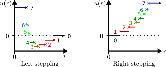
Type="Stepped"

Description

This Potential type allows a stepped potential to be manual entered and is the most general stepped potential available. There are two classes of stepped potential, Left or Right, depending on which "side" of the discontinuity is specified by the discontinuity's energy. An illustration is given below:

A comparison of the two types of stepped potential. The discontinuity locations are marked with a cross, and the adjacent line marks the location of the corresponding step. The internal numbering DynamO uses for each step is also outlined.

In both potentials, there is an implicit step (the zero step) which has an energy of zero. Left stepped potentials are best used for forces which decay with $r$, whereas Right stepped potentials are often used for forces which increase with $r$. This is for efficiency due to two factors: The step number for a pair of particles is not stored in memory if it has a value of zero and, for automatically generated potentials, steps are computed from step 0 upwards (as required). Therefore, a stepped Lennard-Jones potential is most efficiently implemented as a Left potential as most possible particle pairs are not interacting and will be within the zero step. A computed bond (constraining) spring potential is most efficiently implemented using a Right potential.

Example usage

An implementation of the sixth hand stepped approximation of the Lennard-Jones potential reported by Chapela et al. (1989):

<Potential Type="Stepped" Direction="Left">
  <Step R="2.3" E="-0.06"/>
  <Step R="1.75" E="-0.22"/>
  <Step R="1.45" E="-0.55"/>
  <Step R="1.25" E="-0.98"/>
  <Step R="1.05" E="-0.47"/>
  <Step R="1.0" E="0.76"/>
  <Step R="0.95" E="3.81"/>
  <Step R="0.9" E="10.95"/>
  <Step R="0.85" E="27.55"/>
  <Step R="0.80" E="66.74"/>
  <Step R="0.75" E="1.0e+300"/>
</Potential>

Full Tag, Subtag, and Attribute List

Type (attribute): Must have the value "Stepped" to select this Potential type.
Direction (attribute): This sets the direction of the stepping.
For example, for potentials which have zero interaction energy at long distances, the "Left" direction is the most convenient. The Lennard-Jones potential is an example of such a potential. In this case, each Step tag specifies a location of a discontinuity and the energy on its left hand side ($r^-$). The outermost step is assumed to have an energy of zero.
A spring potential is an example where the "Right" direction is most convenient as it has zero interaction energy at $r=0$. In this case, each Step tag specifies a location of a discontinuity and the energy on its right hand side ($r^+$). The innermost step has a energy of zero
Step (tag): This tag represents a single discontinuity/step of the stepped potential. On load these steps are sorted by their R value and allocated numbers as outlined above.
- R (attribute): The radial separation of the discontinuity.
- E (attribute): The energy of the potential on either the left or right hand side of the discontinuity (depending on the Direction).

Type="LennardJones"

Description

This Potential is a stepped approximation to the truncated and shifted Lennard-Jones potential. The approximation and its optimisation is reported in the paper: "Mapping continuous potentials to discrete forms," by Thomson, Lue, and Bannerman. This paper should be consulted for a more detailed discussion of the parameters below. An example of a accurate approximation is given below:

The continuous Lennard-Jones potential and a stepped approximation using the optimal/default settings and $10.8$ attractive steps. Both potentials have a cut-off radius of 3. The figure is in reduced units corresponding to $\varepsilon=1$ and $\sigma=1$

The set-up of this stepped potential is outlined below.

Example usage

<Potential Type="LennardJones" Sigma="1" Epsilon="1" CutOff="3" AttractiveSteps="10.8"/>

Full Tag, Subtag, and Attribute List

Type (attribute): Must have the value "LennardJones" to select this Potential type.
Sigma (attribute): Sets the distance $\sigma$ at which the interaction energy is zero.
Epsilon (attribute): Sets the energy $\varepsilon$ of the attractive well.
Cutoff (attribute): The cutoff radius of the potential.
AttractiveSteps (attribute): The order of approximation of the potential. Setting AttractiveSteps="10.8" is sufficient for a close reproduction of the thermodynamic properties provided the default UMode and RMode values are used.
RMode (attribute, optional): Select the method used to calculate the position of each step. This may be "DeltaR", "DeltaU", or "DeltaV". If this attribute is not set, the default/recommended value is used (currently "DeltaU").
UMode (attribute, optional): Select the method used to calculate the energy of each step. This may be "Left", "Right", "Midpoint", "MidVolume", "Virial", or "Volume". If this attribute is not set, the default/recommended value is used (currently "Volume"). If "Virial" is selected, the Temperature attribute must also be set.
Temperature (attribute, optional): If the UMode is set to "Virial" you must provide the temperature used for the approximation in this attribute.

IDRange

IDRanges are used to specify a range of Particle IDs. These are used in Species, Local, Global and Structure objects to specify the set of particles to which they apply.

Type="All"

Description

An ID Range which maps to all particles in the simulation.

Example usage

<IDRange Type="All"/>

Full Tag, Subtag, and Attribute List

Type (attribute): Must have the value "All" to select this range type.

Type="None"

Description

An ID Range which does not map to any particles.

Example usage

<IDRange Type="None"/>

Full Tag, Subtag, and Attribute List

Type (attribute): Must have the value "None" to select this range type.

Type="Ranged"

Description

An ID Range which maps to a sequential list of particles simulation. The range is inclusive (both its start and end points are inside the range).

Example usage

The following example IDRange includes the particle IDs 0, 1, 2, 3, 4, and 5.

<IDRange Type="Ranged" Start="0" End="5"/>

Full Tag, Subtag, and Attribute List

Type (attribute): Must have the value "Ranged" to select this range type.
Start (attribute): The lowest value ID which is inside the range.
End (attribute): The highest value ID which is inside the range.

Type="List"

Description

An ID Range which maps to a specified list of particles. This is the most general type of Range possible, as all IDs inside the range must be specfied individually.

Example usage

The following example IDRange includes the particle IDs 0, 2, and 5.

<IDRange Type="List">
  <ID val="0"/>
  <ID val="2"/>
  <ID val="5"/>
</IDRange>

Full Tag, Subtag, and Attribute List

Type (attribute): Must have the value "List" to select this range type.
ID (tag): A tag containing an ID/entry in the list.
- val (attribute): The ID of the entry.

Type="Union"

Description

An IDRange which combines several IDRanges into one.

Example usage

<IDRange Type="Union">
  <IDRange .../>
  <IDRange .../>
  ...
</IDRange>

Full Tag, Subtag, and Attribute List

Type (attribute): Must have the value "Union" to select this range type.
IDRange (tag): A list of IDrange subtags which describe the IDRanges to be combined.

IDPairRange

IDPairRanges are used to specify the pairs of particles to which an Interaction applies. Each IDPairRange represent a collection or set of ID pairs.

Type="All"

Description

An ID Range which maps to all pairs of particles in the simulation.

Example usage

<IDPairRange Type="All"/>

Full Tag, Subtag, and Attribute List

Type (attribute): Must have the value "All" to select this range type.

Type="None"

Description

An ID Range which doesn't map to any pair of particles.

Example usage

<IDPairRange Type="None"/>

Full Tag, Subtag, and Attribute List

Type (attribute): Must have the value "None" to select this range type.

Type="Pair"

Description

This creates a IDPairRange from two IDRanges. Each particle ID in the first range is paired with all of the particle IDs in the second range. Pairs of particle IDs which only match one range are not included in the pair range.

Example usage

This example pairs particle IDs 0,1,2 with IDs 3,4,5. Pairs only within one range, such as (0,1) or (3,4), are not included. All IDRangePairs are symmetric, so both (1,4) and (4,1) are included in this example range.

<IDPairRange Type="Pair">
  <IDRange Type="Ranged" Start="0" End="2"/>
  <IDRange Type="Ranged" Start="3" End="5"/>
</IDPairRange>

Full Tag, Subtag, and Attribute List

Type (attribute): Must have the value "Pair" to select this range type.
IDRange ($2\times$tag): There must be two IDRange tags present and each specifies one of the IDRanges used to make the IDPairRange. The order in which the IDRanges are specifed is unimportant. See the section on the available IDRange types for more information.

Type="Single"

Description

This creates a IDPairRange from one IDRange. Every particle ID in the IDRange is paired with every other particle in the IDRange.

Example usage

This example pairs particle IDs 0-0, 0-1, 0-2, 1-1, 1-2, and 2-2.

<IDPairRange Type="Single">
  <IDRange Type="Ranged" Start="0" End="2"/>
</IDPairRange>

Full Tag, Subtag, and Attribute List

Type (attribute): Must have the value "Single" to select this range type.
IDRange (tag): See the section on the available IDRange types for more information.

Type="Self"

Description

This creates a IDPairRange from one IDRange. Every particle ID in the IDRange is paired with itself.

Example usage

This example pairs particle IDs 0-0, 1-1, and 2-2.

<IDPairRange Type="Self">
  <IDRange Type="Ranged" Start="0" End="2"/>
</IDPairRange>

Full Tag, Subtag, and Attribute List

Type (attribute): Must have the value "Self" to select this range type.
IDRange (tag): See the section on the available IDRange types for more information.

Type="List"

Description

This is the most versatile IDPairRange available as it allows you to specify the particle pairings individually.

Example usage

This example matches the particle pairings (0,1), (1,2), and (2,3). As IDPairRanges are symmetric, the pairings (1,0), (2,1), and (3,2) are also included. This example might be used to bond particles together into a chain.

<IDPairRange Type="List">
  <IDPair ID1="0" ID2="1"/>
  <IDPair ID1="1" ID2="2"/>
  <IDPair ID1="2" ID2="3"/>
</IDPairRange>

Full Tag, Subtag, and Attribute List

Type (attribute): Must have the value "List" to select this range type.
IDPair (tag): Each IDPair tag specifies one pairing of particle IDs.
- ID1 (attr): The first ID of the pair. The order of the IDs is unimportant and DynamO always writes the configuration out so that ID1 is the lowest of the pair.
- ID2 (attr): The second ID of the pair.

Type="Union"

Description

This creates a IDPairRange from a combination/union of several IDPairRanges.

Example usage

<IDPairRange Type="Union">
  <IDPairRange .../>
  <IDPairRange .../>
  ...
</IDPairRange>

Full Tag, Subtag, and Attribute List

Type (attribute): Must have the value "Union" to select this range type.
IDPairRange (tag): Each IDPairRange sub tag represents one of the IDPairRanges to be combined.

Type="Chains"

Description

This IDPairRange is provided as a convenient way to bond sequential particle IDs into linear chains.

Example usage

If the example below was used with a square-bond Interaction, it would bond a set of particles together into chains of 4. This example matches the particle pairings (0,1), (1,2), (2,3) and (4,5), (5,6), (6,7). As IDPairRanges are symmetric, the pairings (1,0), (2,1), etc. are also included.

<IDPairRange Type="Chains" Start="0" End="7" Interval="4"/>

Full Tag, Subtag, and Attribute List

Type (attribute): Must have the value "Chains" to select this range type.
Start (attribute): The first ID of the sequential particle IDs.
End (attribute): The last ID of the sequential particle IDs.
Interval (attribute): How long the chains are. Please note that End - Start must be a whole multiple of Interval.

Page last modified: Thursday 29th July 2021